Advent of Code is an annual, pre-Christmas series of programming tasks packaged as an Advent calendar. Behind its doors, daily challenges are hidden, each more difficult than the previous.
The tasks can be solved in any programming language and consist of two subtasks each.
Is Advent of Code Hard?
The first subtask can usually be solved relatively quickly.
In the second task, the scale of the problem is drastically increased. This usually leads to the need to revise the solution since the intuitively implemented algorithm often has too high a complexity class and would take hours, days, or even months to solve the task.
Shortly after the release of a new Advent of Code puzzle, you can find the first solutions on the corresponding Reddit. Those solutions primarily consist of procedural spaghetti code that is not very readable, let alone maintainable.
My Advent of Code Answers 2022
I, therefore, took the trouble to implement each task in Java in a genuinely object-oriented and test-driven way, resulting in a solution of small, understandable objects interacting with each other.
This approach also usually results in the optimizations required for subtask two being limited to a small section of the code – often a single class.
To calculate the sum of the three largest blocks, we need to sort the stream in descending order. Unfortunately, this requires boxing and unboxing since an IntStream can only be sorted in ascending order:
On day 2, we have to write a simulator for Rock paper scissors. I solved subtask two, where we have to infer the move from the game result by trial and error – there are only three possible moves after all. Of course, it would be more elegant to calculate the player’s move from the combination of the opponent’s move and the desired result.
On day 3, we need to implement an algorithm that filters out those items that occur multiple times from multiple lists of items (from two compartments of a backpack or three backpacks).
Comparing each element of one list with all elements of the two other lists would result in a time complexity of O(n²).
Since the set of possible elements (A-Z and a-z) is very small, we can instead create an array of bitsets for each possible element, then iterate over each list and set a bit for the corresponding list for each element it contains, and finally check for which elements all bits are set. This algorithm has a significantly better time complexity O(n).
For day 4, I implemented the class SectionAssignment. It stores the start and end point of a section and provides methods to check if one section fully contains another or if two sections partially overlap:
record SectionAssignment(int start, int end){
booleanfullyContains(SectionAssignment other){
return start <= other.start && end >= other.end;
}
booleanoverlaps(SectionAssignment other){
return start >= other.start && start <= other.end
|| end >= other.start && end <= other.end
|| other.start >= start && other.start <= end
|| other.end >= start && other.end <= end;
}
}Code language:Java(java)
With this class, both subtasks are quickly solved.
On day 5, I applied the Strategy Pattern to implement the two types of cranes and make them interchangeable:
The move() methods are implemented as follows. The CrateMover 9000 takes – one by one – the desired number of crates from one stack and places them on the other:
classCrateMover9000implementsCrateMover{
@Overridepublicvoidmove(CrateStacks crateStacks, Move move){
CrateStack fromStack = CrateMover.getSourceStack(crateStacks, move);
CrateStack toStack = CrateMover.getTargetStack(crateStacks, move);
for (int i = 0; i < move.number(); i++) {
toStack.push(fromStack.pop());
}
}
}Code language:Java(java)
CrateMover 9001 uses an auxiliary stack to flip the order of the crates in between:
classCrateMover9001implementsCrateMover{
@Overridepublicvoidmove(CrateStacks crateStacks, Move move){
CrateStack fromStack = CrateMover.getSourceStack(crateStacks, move);
CrateStack toStack = CrateMover.getTargetStack(crateStacks, move);
Deque<Crate> helperStack = new LinkedList<>();
for (int i = 0; i < move.number(); i++) {
helperStack.push(fromStack.pop());
}
while (!helperStack.isEmpty()) {
toStack.push(helperStack.pop());
}
}
}Code language:Java(java)
I implemented the solution for day 6 using a Set<Character>. From each position in the string, we write the preceding characters, according to the marker length, to the Set. As soon as we encounter a character the Set already contains, we clear the Set and repeat the attempt at the next character – until we find the marker (i.e., the required number of different characters).
For day 7, I wrote a parser that builds a directory tree from the given commands using the following classes (conforming to the composite pattern):
For the solution of part one, we then only need to recursively go through all subdirectories and filter out those that match the size criterion. We can solve this very elegantly with Java’s Stream API:
To solve the task for day 8, we don’t need any tricks, just some programming work. We can do a lot for the code’s readability by modeling directions as an enum and positions as a record (the moveTo(…) method is implemented using the Switch Expression introduced in Java 14):
enum Direction {
TOP,
RIGHT,
BOTTOM,
LEFT;
}
record Position(int column, int row){
Position moveTo(Direction direction){
returnswitch (direction) {
case TOP -> new Position(column, row - 1);
case RIGHT -> new Position(column + 1, row);
case BOTTOM -> new Position(column, row + 1);
case LEFT -> new Position(column - 1, row);
};
}
}Code language:Java(java)
Using Position.moveTo(…), we can then walk from each field to the four cardinal directions and match the height of the trees with the criteria of the respective subtask.
On day 10, we need to implement a simple CPU emulator that can perform two different operations and turn a pixel on a screen on or off during the duration of these operations according to the X register and the screen’s current X position. The implementation does not require any tricks or optimizations.
The problem with part two of day 11 is that the “worry level” quickly takes on gigantic proportions due to squaring. The trick to keep the worry level low without changing the game logic is to replace the relief formula
where reliefDivisor is the product of all the different denominators of the “test” operations.
In the example, we have the following four tests:
Test: divisible by 23
Test: divisible by 19
Test: divisible by 13
Test: divisible by 17Code language:plaintext(plaintext)
For this example, the reliefDivisor is calculated as 23 × 19 × 13 × 17 = 96,577
If we now, for the relief operation, set the worry level to the remainder when dividing by this value, it is ensured that a) the worry level remains small and b) the result of the “test” operations do not change, no matter which monkey has a specific item.
For day 12, I implemented a breadth-first algorithm that goes from the start position to all reachable fields and then from each reachable field further to all fields reachable from there, and so on. Fields already reached in a previous step are ignored since a shorter path has already been found there.
For part two, I simply applied the algorithm from part one to all possible starting squares and determined the shortest of all shortest paths.
The relatively small size of the problem made this trivial solution possible. If the map had been much larger, it would have been possible to go back from the finish to the start and return the squares traversed up to that point when reaching a potential start square for the first time.
For day 13, I wrote a Comparator that I use both in part one to count how many packet pairs are in the correct order and in part two to sort the packets using List.sort().
The trivial solution for day 15 also works with a grid. For part two, however, a grid proves to be too costly.
The trick is to store the areas covered by the sensors not in a grid but with start and end positions, combining adjacent or overlapping regions and ultimately determining the uncovered position from these regions.
The task of day 16 can be solved with a depth-first search. There is not one optimization but several, each of which makes the algorithm faster by a significant factor. I applied the following four optimizations:
In each situation, the algorithm checks whether the same situation (i.e., the combination of valve positions, actuator positions, and elapsed minutes) has occurred before. If so, and if that situation resulted in the same or more pressure being discharged, the current path does not need to be explored further.
In each situation, the maximum amount of pressure that can be released during the remaining time if the valves are opened according to descending flow rate is calculated. If this results in a worse result than the current best, the path is not pursued further.
When comparing the situation with all previous situations, two situations are considered the same even if the positions of you and the elephant are reversed.
If it is detected that an actor has run in a circle without having opened a valve on it, the current path is also not followed further.
With the help of these optimizations, sub-task two can be solved in about two seconds.
The simulation for day 17 is implemented relatively quickly with binary operations: “shift left” and “shift right” to move the rock, “bitwise and” for collision checking, and “bitwise or” for manifesting a rock.
However, simulating 1,000,000,000 rocks would have taken close to 20 hours with my initial implementation.
The trick for subtask two is to find repetitions in the fall and displacement patterns. To do this, my algorithm stores a combination of the current rock, the current position in the input, and the height profile of the upper rock rows as a key in a map with the current highest rock and the number of rocks that have fallen so far as the value.
As soon as the same combination occurs again (which happens surprisingly quickly), we can skip a few billion steps in a few milliseconds with the help of the number of rocks that have fallen in the meantime and the intermediate growth of the rock mountain. Thus, subtask two can also be solved in a few hundred milliseconds.
Subtask one of day 18 is quickly solved. We store all cubes in a set and then iterate over it and count – using Set.contains() – those sides on which there is no cube.
I solved part two with iterative floodfill. The area outside the droplet is filled cube by cube with “steam.” Each time a cube cannot be filled because there is lava, a counter is incremented. In the end, this counter contains the searched outer area.
Day 19 reminds us of the valve task from day 16. This task is also solved with a depth-first search and various optimizations:
Assuming that we produce a geode robot every turn, we can calculate the maximum number of geodes that could still be produced in a given situation. If this number is smaller than the current best value, the path does not need further exploration.
If a certain robot could have been bought in the previous round – but no robot was bought in that round, then we don’t need to buy it now. Saving only makes sense for another robot.
At the last minute, we do not need to produce a robot.
In the penultimate minute, we only need to produce geode robots.
In the pre-penultimate minute, we only need to produce geode, ore, or obsidian robots (i.e., no clay robots).
My implementation solves part one in 4 seconds and part two in 52 seconds.
The solution for day 20 can be implemented easily with a doubly linked circular list. Part one does not require any optimizations.
In part two, we would have to move the nodes several trillion times. We can reduce that to a few thousand with a simple formula:
long distance = node.value() % (size - 1);Code language:Java(java)
The trick is not to divide by size (the number of elements) but by size - 1. You can see this in the example: In the list of length 7, you would have to move an element six times to the right to get it back to its starting point.
For the solution of day 21, I built a directed acyclic graph of the mathematical operations. Since the results of some operations are used multiple times, they are stored once they have been calculated.
For part two, I first tried to implement a depth-first search, i.e., using different values for the “humn” node and then checking whether both operands of the “root” node are the same. I optimized this variant by not deleting all stored results between two attempts but only those on the path from “root” to “humn.” But even so, the calculation would have taken too long to accept this solution.
Based on the optimization just mentioned, I was able to implement a much faster solution. We can simply execute the mathematical operations on the path from “root” to “humn” backwards and get the result in a few milliseconds.
Day 22 started off easy once again. With a two-dimensional grid and a few special treatments for the areas outside the map, part one is quickly solved.
Part two is much trickier. I wrote logic for this that maps the coordinates on the map to coordinates on a cube face, then moves and rotates the cube face using an additional list of edge connections (“wormholes”), and finally maps the coordinates on the moved and rotated cube face back to the coordinates on the global map.
I manually generated the list of edge connections from my puzzle input. So my solution will not work without manually adjusting the edge connections on all of them (unless your input has the same cutting pattern). You can also determine the edge connections algorithmically, but I haven’t had time to do that. I may do that later.
On day 23, when solving the first sub-task, we can already be prepared that we will probably have to simulate more than ten rounds in sub-task two. Since the field will keep growing this way, we should not store the elves in a two-dimensional array.
My algorithm stores the elves as a list and additionally their positions in a Set<Position>. So the collision check can be easily solved via Set.contains(). Solving subtask two takes less than one second.
On day 24, we once more have to implement a pathfinding algorithm. For today’s task, a depth-first search is not suitable because the map changes with each move. With my puzzle input, it takes 95,400 steps to reach the target the first time and just over a minute to solve subtask one.
A breadth-first search solves part one in just 95 ms and part two in 130 ms.
I optimized the calculation of free positions. Instead of simulating the complete valley map for each step, I use a modulo operation to calculate whether a field is free at a certain time or not:
The solution for day 25 consists of only a few lines of code. The trickier part is converting a decimal number to a SNAFU string. This is the corresponding method:
static String toSnafuString(long decimal){
StringBuilder result = new StringBuilder();
do {
long fives = (decimal + 2) / 5;
int digit = (int) (decimal - 5 * fives);
result.insert(0, convertDecimalToSnafuDigit(digit));
decimal = fives;
} while (decimal != 0);
return result.toString();
}Code language:Java(java)
If you liked the article, please share it using one of the share buttons at the end. Want to be notified by email when I publish a new article? Then click here to join the HappyCoders newsletter.
In this article, you will learn about the “Radix Sort” sorting algorithm. You will learn:
How does Radix Sort work? (Step by step)
How to implement Radix Sort in Java?
What is the time and space complexity of Radix Sort?
What variants of Radix Sort exist?
… and what does the term “radix” mean anyway?
Let’s start with the last question:
What is Radix Sort?
“Radix” is the Latin word for “root” – nevertheless, Radix Sort has nothing to do with calculating square roots.
Instead, the “radix” of a number system (also called the “base”) refers to the number of digits needed to represent numbers in that number system. The radix in the decimal system is 10, the radix of the binary system is 2, and the radix of the hexadecimal system is 16.
In Radix Sort, we sort the numbers digit by digit – and not, as in most other sorting methods, by comparing two numbers. You can read more about how this works in the following chapter.
Radix Sort Algorithm
The algorithm for Radix Sort is best explained step by step using an example. We want to sort the following numbers:
We will start by looking at the last digit only (there are also Radix Sort variations where you start at the first digit, but we’ll get to that later):
We sort the numbers in two phases: a partitioning phase and a collection phase.
Partitioning Phase
For the partitioning, we create ten so-called “buckets”, designated with “0” to “9”. We distribute the numbers to these buckets according to their last digit. The following image demonstrates how we place the first number, 41, in bucket “1”:
The second number, 573, is placed in bucket “3” according to its last digit:
The third number, 3, is also placed in bucket “3”:
In the same way, we distribute the remaining numbers to the buckets:
That completes the partitioning phase for the last digit.
Collection Phase
The partitioning phase is followed by the collecting phase. We collect the numbers, bucket by bucket, in ascending order – and within the buckets from left to right (i.e., in the same order as the numbers were entered in the respective bucket) – into a new list.
We start with the bucket with the smallest digit, i.e., bucket 1:
After that, we collect the numbers of the next higher bucket, that’s bucket 3:
And finally, the numbers from bucket 6 and then bucket 8:
All buckets are now empty:
In this new list, the numbers are sorted in ascending order by their last digit: 1, 1, 3, 3, 6, 8
Sorting by Tens Place
We repeat the partitioning and collecting phase for the tens place digits. This time, I represent the two phases with only one image each.
In the partitioning phase, we distribute the numbers to the buckets according to their tens place digit:
The tens place digit of one-digit numbers is zero. Accordingly, I have represented the three as “03”.
In the collection phase, we again collect the numbers, bucket by bucket:
The numbers are now sorted according to their last two digits: 3, 8, 36, 41, 71, 73, 93
Sorting by Hundreds Place
We repeat the same procedure for the hundreds place. First, the partitioning phase:
And after that, the collection phase:
After the third and final collection phase, the numbers are entirely sorted.
Here again, are the final result without leading zeros:
In the next chapter, we come to the implementation of Radix Sort.
Radix Sort in Java
Radix Sort can be implemented in several ways. We’ll start with a simple variant that is very close to the algorithm described. After that, I will show you two alternative implementations.
Variant 1: Radix Sort With Dynamic Lists
We start with an empty sort() method and fill it step by step.
(You can find the final result at the end of this section and in the RadixSortWithDynamicLists class in the GitHub repository of this sorting tutorial series).
public class RadixSortWithDynamicLists
publicvoidsort(int[] elements){
// We will implement this method step by step...
}
}Code language:Java(java)
Since we need to repeat the two phases (partitioning phase and collecting phase) for each digit, we first need to determine how many digits our numbers have.
We do this by finding the largest number from the array to be sorted and then counting how many times that number can be divided by 10:
public class RadixSortWithDynamicLists
publicvoidsort(int[] elements){
int max = getMaximum(elements);
int numberOfDigits = getNumberOfDigits(max);
// TODO: Implement the partitioning and collection phases
}
privatestaticintgetMaximum(int[] elements){
int max = 0;
for (int element : elements) {
if (element > max) {
max = element;
}
}
return max;
}
privateintgetNumberOfDigits(int number){
int numberOfDigits = 1;
while (number >= 10) {
number /= 10;
numberOfDigits++;
}
return numberOfDigits;
}
}Code language:Java(java)
Then we sort digit by digit. We write a for loop with the loop variable digitIndex, where 0 stands for the units place, 1 for the tens place, 2 for the hundreds place, and so on.
(In the following listings, I don’t print the class anymore, only the methods within the class).
publicvoidsort(int[] elements){
int max = getMaximum(elements);
int numberOfDigits = getNumberOfDigits(max);
for (int digitIndex = 0; digitIndex < numberOfDigits; digitIndex++) {
// TODO: Sort elements by digit at 'digitIndex'
}
}Code language:Java(java)
For the next step, we need the buckets to distribute the numbers to. We could use ten ArrayLists for this.
However, it is more elegant to wrap them in a Bucket class. That makes the code more readable and allows us to change the implementation of the buckets later without having to change the rest of the code.
We can create the Bucket class as an inner class inside RadixSortWithDynamicLists:
privatestaticclassBucket{
privatefinal List<Integer> elements = new ArrayList<>();
privatevoidadd(int element){
elements.add(element);
}
private List<Integer> getElements(){
return elements;
}
}Code language:Java(java)
That was the preparation.
Let’s move on to the partitioning phase. We need ten buckets on which to distribute the numbers; we generate them with a createBuckets() method:
private Bucket[] createBuckets() {
Bucket[] buckets = new Bucket[10];
for (int i = 0; i < 10; i++) {
buckets[i] = new Bucket();
}
return buckets;
}Code language:Java(java)
After that, we distribute our numbers among the buckets based on the digit at the digitIndex currently under consideration:
privatevoiddistributeToBuckets(int[] elements, int digitIndex, Bucket[] buckets){
int divisor = calculateDivisor(digitIndex);
for (int element : elements) {
int digit = element / divisor % 10;
buckets[digit].add(element);
}
}
privateintcalculateDivisor(int digitIndex){
int divisor = 1;
for (int i = 0; i < digitIndex; i++) {
divisor *= 10;
}
return divisor;
}Code language:Java(java)
The divisor is the number by which we must divide an element so that the rearmost digit is the digit currently under consideration – i.e., 1 for the units place, 10 for the tens place, 100 for the hundreds place, and so on.
We combine the methods of the partitioning phase in a partition() method:
And now, we close the circle by calling the sortByDigit() method from the digitIndex loop in the sort() method shown at the beginning:
publicvoidsort(int[] elements){
int max = getMaximum(elements);
int numberOfDigits = getNumberOfDigits(max);
for (int digitIndex = 0; digitIndex < numberOfDigits; digitIndex++) {
sortByDigit(elements, digitIndex);
}
}Code language:Java(java)
That completes our Radix Sort implementation.
Here you can see the complete source code again:
publicclassRadixSortWithDynamicLists{
publicvoidsort(int[] elements){
int max = getMaximum(elements);
int numberOfDigits = getNumberOfDigits(max);
for (int digitIndex = 0; digitIndex < numberOfDigits; digitIndex++) {
sortByDigit(elements, digitIndex);
}
}
privatestaticintgetMaximum(int[] elements){
int max = 0;
for (int element : elements) {
if (element > max) {
max = element;
}
}
return max;
}
privateintgetNumberOfDigits(int number){
int numberOfDigits = 1;
while (number >= 10) {
number /= 10;
numberOfDigits++;
}
return numberOfDigits;
}
privatevoidsortByDigit(int[] elements, int digitIndex){
Bucket[] buckets = partition(elements, digitIndex);
collect(buckets, elements);
}
private Bucket[] partition(int[] elements, int digitIndex) {
Bucket[] buckets = createBuckets();
distributeToBuckets(elements, digitIndex, buckets);
return buckets;
}
private Bucket[] createBuckets() {
Bucket[] buckets = new Bucket[10];
for (int i = 0; i < 10; i++) {
buckets[i] = new Bucket();
}
return buckets;
}
privatevoiddistributeToBuckets(int[] elements, int digitIndex, Bucket[] buckets){
int divisor = calculateDivisor(digitIndex);
for (int element : elements) {
int digit = element / divisor % 10;
buckets[digit].add(element);
}
}
privateintcalculateDivisor(int digitIndex){
int divisor = 1;
for (int i = 0; i < digitIndex; i++) {
divisor *= 10;
}
return divisor;
}
privatevoidcollect(Bucket[] buckets, int[] elements){
int targetIndex = 0;
for (Bucket bucket : buckets) {
for (int element : bucket.getElements()) {
elements[targetIndex] = element;
targetIndex++;
}
}
}
privatestaticclassBucket{
privatefinal List<Integer> elements = new ArrayList<>();
privatevoidadd(int element){
elements.add(element);
}
private List<Integer> getElements(){
return elements;
}
}
}Code language:Java(java)
By the way, the RadixSortWithDynamicLists class in the GitHub repository is slightly different from the source code printed here:
It implements the SortAlgorithm interface, which allows comparison of different Radix Sort implementations with each other and with the other algorithms of the sorting algorithm series.
The getMaximum() method is placed in the ArrayUtils class.
The getNumberOfDigits() and calculateDivisor() methods are in the RadixSortHelper class and can thus be used in other Radix Sort implementations.
The implementation shown has one shortcoming:
Dynamic lists (i.e., lists that can change size at runtime) are not optimal for performance-critical purposes such as sorting algorithms because adding elements involves some performance overhead (for example, in a linked list, new nodes must be created; in an ArrayList, the array must be recopied into a larger one at certain intervals).
In the next section, I will show you an alternative variant.
Variant 2: Radix Sort with Arrays
We can speed up the implementation significantly (we will compare the performance of the implementations afterward) by using an array instead of an ArrayList for the buckets.
Since arrays have a fixed size, we need to know how many elements a bucket will contain before creating it. We modify our Bucket class as follows and pass the size to its constructor:
To determine how many elements a bucket should contain, we first count the digits at the current digitIndex. The partition() method then looks like this:
private Bucket[] partition(int[] elements, int digitIndex) {
int[] counts = countDigits(elements, digitIndex);
Bucket[] buckets = createBuckets(counts);
distributeToBuckets(elements, digitIndex, buckets);
return buckets;
}
privateint[] countDigits(int[] elements, int digitIndex) {
int[] counts = newint[10];
int divisor = calculateDivisor(digitIndex);
for (int element : elements) {
int digit = element / divisor % 10;
counts[digit]++;
}
return counts;
}
private Bucket[] createBuckets(int[] counts) {
Bucket[] buckets = new Bucket[10];
for (int i = 0; i < 10; i++) {
buckets[i] = new Bucket(counts[i]);
}
return buckets;
}Code language:Java(java)
We don’t need to change the distributeToBuckets() method or any other method shown in variant 1. Good thing we used a Bucket class in the first variant – and not an ArrayList :-)
You can find the complete code of variant 2 in the RadixSortWithArrays class in the GitHub repository.
Let’s move on to a third variant.
Variant 3: Radix Sort with Counting Sort
In variant 2, we counted in advance how many elements would be sorted into each bucket. With this information, we can skip the buckets and move the elements directly to their target positions. We do this by applying the general form of Counting Sort.
I won’t repeat here how Counting Sort works. I’ll show you the implementation right away:
publicclassRadixSortWithCountingSort{
@Overridepublicvoidsort(int[] elements){
int max = getMaximum(elements);
int numberOfDigits = getNumberOfDigits(max);
// Remember input arrayint[] inputArray = elements;
for (int digitIndex = 0; digitIndex < numberOfDigits; digitIndex++) {
elements = sortByDigit(elements, digitIndex);
}
// Copy sorted elements back to input array
System.arraycopy(elements, 0, inputArray, 0, elements.length);
}
// Same as in the other variants:// getMaximum(), getNumberOfDigits(), calculateDivisor() privateint[] sortByDigit(int[] elements, int digitIndex) {
int[] counts = countDigits(elements, digitIndex);
int[] prefixSums = calculatePrefixSums(counts);
return collectElements(elements, digitIndex, prefixSums);
}
privateint[] countDigits(int[] elements, int digitIndex) {
int[] counts = newint[10];
int divisor = calculateDivisor(digitIndex);
for (int element : elements) {
int digit = element / divisor % 10;
counts[digit]++;
}
return counts;
}
privateint[] calculatePrefixSums(int[] counts) {
int[] prefixSums = newint[10];
prefixSums[0] = counts[0];
for (int i = 1; i < 10; i++) {
prefixSums[i] = prefixSums[i - 1] + counts[i];
}
return prefixSums;
}
privateint[] collectElements(int[] elements, int digitIndex, int[] prefixSums) {
int divisor = calculateDivisor(digitIndex);
int[] target = newint[elements.length];
for (int i = elements.length - 1; i >= 0; i--) {
int element = elements[i];
int digit = element / divisor % 10;
target[--prefixSums[digit]] = element;
}
return target;
}
}Code language:Java(java)
There are two basic variants of Radix Sort, which differ in the order in which we look at the digits of the elements.
LSD Radix Sort
The Radix Sort algorithm shown in the first chapter is called “LSD Radix Sort”. LSD stands for “least significant digit”. We started sorting at the least significant digit (the ones) and worked our way up, digit by digit, to the most significant digit.
MSD Radix Sort
Alternatively, we can also start at the most significant digit. Accordingly, the second variant is called “MSD Radix Sort”.
However, we have to proceed differently than with the LSD variant. Because if we were to sort the entire input list in our initial example first by hundreds place, then by tens place, and finally by units place, the following would happen (I have omitted the buckets in the graphic since we are only concerned with the results after the three collect phases):
Sorting by the tens place and ones place has mixed up the respective previous sortings.
The problem is solved quickly:
After the hundreds place, we must not sort the input list again as a whole, but the hundreds place buckets within themselves. We then sort the resulting tens place buckets by the units place. In other words, we sort the buckets recursively.
MSD Radix Sort – Step by Step
The following diagrams show the recursive MSD Radix Sort procedure step by step using the initial example. Buckets are represented by brackets under the elements. Empty buckets are not shown.
We start with partitioning by hundreds place:
Now, instead of moving from the partitioning phase to the collecting phase, we perform another partitioning phase on each bucket – on the next lower digit, that is, the tens place.
Empty buckets and those containing only one element (such as the 271 and the 836) need not be partitioned further.
Actually, we would now have to partition the buckets by units place. But since none of the tens place buckets contains more than one element, this is unnecessary.
We, therefore, exit the recursion. First, we execute a collection phase on the tens place buckets:
And lastly, we perform the collection phase on the hundreds place buckets:
That completes the sorting.
MSD Radix Sort – Implementation
Like the LSD variant, we can implement MSD Radix Sort with dynamic lists, arrays, and Counting Sort.
I’ll show you how to modify the LSD array implementation shown above into an MSD implementation with just a few changes.
Here are once more the sort() and sortByDigit() methods of the RadixSortWithArrays class:
publicvoidsort(int[] elements){
int max = getMaximum(elements);
int numberOfDigits = getNumberOfDigits(max);
for (int digitIndex = 0; digitIndex < numberOfDigits; digitIndex++) {
sortByDigit(elements, digitIndex);
}
}
privatevoidsortByDigit(int[] elements, int digitIndex){
Bucket[] buckets = partition(elements, digitIndex);
collect(buckets, elements);
}Code language:Java(java)
All we have to do now is call the sortByDigit() method for the most significant digit first and insert the recursive call for the next lower digit between the partitioning and collecting phases:
publicvoidsort(int[] elements){
int max = getMaximum(elements);
int numberOfDigits = getNumberOfDigits(max);
sortByDigit(elements, numberOfDigits - 1);
}
privatevoidsortByDigit(int[] elements, int digitIndex){
Bucket[] buckets = partition(elements, digitIndex);
// If we haven't reached the last digit, // sort the buckets by the next digit, recursivelyif (digitIndex > 0) {
for (Bucket bucket : buckets) {
if (bucket.needsToBeSorted()) {
sortByDigit(bucket.getElements(), digitIndex - 1);
}
}
}
collect(buckets, elements);
}Code language:Java(java)
The Bucket.needsToBeSorted() method returns true if the bucket contains at least one element.
As an exercise, I’ll leave it to you to write an MSD variant for each of the other two LSD implementations (dynamic lists and Counting Sort).
Using Other Bases
So far, we have partitioned according to the decimal system, i.e., with ten buckets. However, we can also work with any other base, for example, with the binary system (2 buckets), the hexadecimal system (16 buckets), or even with a hundred, a thousand, or more buckets.
The higher the base, the more buckets, and the more complex the partitioning phase. On the other hand, the numbers to sort have fewer digits (1,000,000 decimal = F4240 hexadecimal), so altogether fewer partitioning and collecting phases are required. We will determine what this means for performance in the “Radix Sort Runtime” chapter.
How do you implement Radix Sort with a different base?
Basically, we need to replace each occurrence of the number 10 in the source code with the new base. In the RadixSortWithDynamicLists class, “10” occurs in the following methods:
privateintgetNumberOfDigits(int number){
int numberOfDigits = 1;
while (number >= 10) {
number /= 10;
numberOfDigits++;
}
return numberOfDigits;
}
private Bucket[] createBuckets() {
Bucket[] buckets = new Bucket[10];
for (int i = 0; i < 10; i++) {
buckets[i] = new Bucket();
}
return buckets;
}
privatevoiddistributeToBuckets(int[] elements, int digitIndex, Bucket[] buckets){
int divisor = calculateDivisor(digitIndex);
for (int element : elements) {
int digit = element / divisor % 10;
buckets[digit].add(element);
}
}
privateintcalculateDivisor(int digitIndex){
int divisor = 1;
for (int i = 0; i < digitIndex; i++) {
divisor *= 10;
}
return divisor;
}Code language:Java(java)
We can replace the “10” in all these places with another base. Better yet, we replace it with a variable so that we can invoke the sorting algorithm with any base.
publicclassRadixSortWithDynamicListsAndCustomBaseimplementsSortAlgorithm{
privatefinalint base;
publicRadixSortWithDynamicListsAndCustomBase(int base){
this.base = base;
}
// All methods not printed here are the same as in RadixSortWithDynamicListsprivateintgetNumberOfDigits(int number){
int numberOfDigits = 1;
while (number >= base) {
number /= base;
numberOfDigits++;
}
return numberOfDigits;
}
private Bucket[] createBuckets() {
Bucket[] buckets = new Bucket[base];
for (int i = 0; i < base; i++) {
buckets[i] = new Bucket();
}
return buckets;
}
privatevoiddistributeToBuckets(int[] elements, int digitIndex, Bucket[] buckets){
int divisor = calculateDivisor(digitIndex);
for (int element : elements) {
int digit = element / divisor % base;
buckets[digit].add(element);
}
}
privateintcalculateDivisor(int digitIndex){
int divisor = 1;
for (int i = 0; i < digitIndex; i++) {
divisor *= base;
}
return divisor;
}
}Code language:Java(java)
Please note that in the GitHub repository, the getNumberOfDigits() and calculateDivisor() methods are located in the RadixSortHelper class, as other Radix Sort implementations also use them.
In the GitHub repository, you can also find the adapted algorithms for arrays, Counting Sort, and recursive MSD Radix Sort:
In this chapter, I will show you how to determine the time complexity of Radix Sort. For an introduction to time complexity, see the article “Big O Notation and Time Complexity“.
We use the following variables below:
n = the number of elements to sort
k = the maximum key length (number of digit places) of the elements to sort
b = the base (= the number of buckets)
The algorithm iterates over k digit places; for each place, it performs the following operation:
It creates b buckets. The cost of this is constant in each case.
It iterates over all n elements to sort them into the buckets. The cost of calculating a bucket number and inserting an element into a bucket is constant.
It iterates over b buckets and copies a total of n elements from them. The cost for each of these steps is again constant.
We ignore constant parts in the determination of the time complexity. This results in:
The time complexity for Radix Sort is: O(k · (b + n))
The cost is independent of how the input numbers are arranged. Whether they are randomly distributed or pre-sorted makes no difference to the algorithm. Best case, average case, and worst case are, therefore, identical.
The formula looks complicated at first. But two of the three variables are not variable in most situations. For example, if we sort longs with a base of 10, we can replace k with 19 (the maximum possible value for a long is 9,223,372,036,854,775,807) and b with 10.
The formula then becomes O(19 · (10 + n)). We can omit constants; thus, we get:
The time complexity for Radix Sort with a known maximum length of the elements to sort and with a fixed base is: O(n)
So, for primitive data types like integer and long (for these, we know the maximum length), Radix Sort has a better time complexity than Quicksort!
You’ll find out whether Radix Sort is actually faster in the next chapter. We will measure the runtime of the various Radix Sort implementations and compare them with each other (and with Quicksort).
Radix Sort Runtime
In this chapter, I’ll show you the results of some performance tests I ran using the UltimateTest and CompareRadixSorts tools to compare the performance of different algorithms, implementations, and bases.
Runtime of Different Radix Sort Implementations
The first diagram shows the comparison of the different implementations:
As expected, the implementation with dynamic lists performs worst. The remaining three variants are in a neck-and-neck race, which the Counting Sort implementation wins by a narrow margin, closely followed by the array variant.
We can also see the linear running time O(n) in each case, which we predicted in the previous chapter.
Effect of the Base on the Runtime
The second diagram shows how the choice of the base affects the runtime of the array implementation:
We can see that the runtime is significantly better for bases of 100 and 1,000 than for smaller and larger bases.
Let’s examine this in a little more detail… The third diagram shows finer gradations of the bases with a fixed number of elements (n = 5,555,555):
Both too small and too large a base are bad for performance.
A very small base leads to many iterations. A base that is too large leads to fewer iterations but significantly more buckets within the iterations.
A sweet spot shows up at a base of 256.
Radix Sort vs. Quicksort
In the following diagram, you can see the runtimes…
of the Radix Sort array implementation with a base of 256,
of dual-pivot Quicksort combined with insertion sort (the fastest variant we determined in the Quicksort tutorial), and
of the JDK sort method Arrays.sort(), which also implements an optimized dual-pivot Quicksort.
And indeed, Radix Sort is not only faster in theory – O(n) vs. O(n log n) – but also in practice – comparing it with both the home-implemented Quicksort and the even faster JDK Quicksort implementation Arrays.sort().
So if you need to sort int primitives and performance is critical, you should consider using Radix Sort instead of Java’s native Arrays.sort(). Feel free to use the implementation from this article.
That is not true for long primitives. For longs, Arrays.sort() is about 50% faster than my Radix Sort implementation.
Other Characteristics of Radix Sort
In this concluding chapter, we consider the space complexity, stability, and parallelizability of Radix Sort, as well as its differences from Counting Sort and Bucket Sort.
Radix Sort Space Complexity
All variants shown in this article require additional memory:
O(b) for the digit counters (not needed in the dynamic lists variant)
O(b) for the bucket references (not required for the counting-sort variant).
O(n) for the contents of the buckets (not needed for the counting-sort variant)
O(n) for an additional target array (only for the Counting Sort variant)
Each variant thus contains at least one O(b) component and at least one O(n) component.
We can therefore conclude:
The space complexity of Radix Sort is: O(b + n)
There is one exception: recursive MSD Radix Sort with base 2 can do without additional memory for the elements by partitioning them in such a way that by exchanging two elements at a time, all elements whose bit is 1 at the currently considered place are pushed to the right side, and all elements whose bit is 0 are pushed to the left side (similar to Quicksort).
Is Radix Sort Stable?
You can read about the definition of stability in sorting methods in the linked introductory article. In short: elements with the same key keep their original order to each other during sorting.
All Radix Sort implementations shown in this article are stable.
In contrast, the in-place MSD Radix Sort variant discussed in the previous section is not stable (analogous to Quicksort).
Parallel Radix Sort
Both Radix Sort variants (LSD and MSD) can be parallelized.
Parallel MSD Radix Sort
With MSD Radix Sort, after the initial partitioning phase, we can sort all the resulting buckets independently in parallel. Thanks to parallel streams, this is very easy to implement in Java:
To parallelize LSD Radix Sort, we need to put a little more effort:
We divide the input array into segments to be processed in parallel (e.g., according to the number of CPU cores).
We calculate in parallel per segment how many elements have to be sorted into which buckets.
When step 2 is complete for all segments, we compute a) per bucket, the total number of elements, and b) per segment, the initial write positions for each bucket.
We distribute the elements from the segments to the buckets in parallel. Using the initial write positions calculated in step 3, we know at which positions within the buckets we must write from which segments.
When step 4 is complete for all segments, we compute per bucket the offset in the target array (as prefix sums over the number of elements in the buckets).
We collect the elements from the buckets in parallel. Using the offsets calculated in step 5, we know at which position in the target array the elements of a bucket must start.
You can find the source code in the ParallelRadixSortWithArrays class in the GitHub repo. The six steps above are marked in the code with correspondingly numbered comments.
Parallel vs. Sequentiell Radix Sort
The following diagram shows the runtime of the parallel variants compared to the sequential variants on a 6-core i7 CPU:
The parallel variants are only about 2.3 times faster, with 67 million elements. That is not even close to factor 6, partly because parts of the code cannot be executed in parallel and partly because the CPU cores have to exchange a lot of data with the main memory (the input array occupies 1 GB).
If we look at a smaller section of the diagram, things look different:
With “only” half a million elements, the parallel Radix Sort variant with arrays is 5.75 times faster than the sequential variant. The CPU cores are almost entirely utilized. That is because the input array is only 2 MB, and the sorting can take place completely in the CPU’s L3 cache.
Radix Sort vs. Counting Sort
Both sorting methods use buckets for sorting. With Counting Sort, we need one bucket for each value. For example, if we wanted to sort integers, we would need about four billion buckets. With Radix Sort, on the other hand, the number of buckets corresponds to the chosen base.
In Radix Sort, we sort iteratively digit by digit; in Counting Sort, we sort the elements in a single iteration.
Counting Sort is therefore primarily suitable for small number spaces.
Radix Sort vs. Bucket Sort
Bucket Sort first distributes items across a given number of buckets such that all items in each bucket are greater than all items in the previous bucket (e.g., 0-99, 100-199, 200-299, etc.).
After that, each bucket is sorted in itself – either recursively with Bucket Sort – or with another sorting method (which exactly is not specified). Finally, the elements from the sorted buckets are joined.
If this sounds familiar to you – you’ve met one form of Bucket Sort in this article: recursive MSD Radix Sort.
Summary
Radix Sort is a stable sorting algorithm with a general time complexity of O(k · (b + n)), where k is the maximum length of the elements to sort (“key length”), and b is the base.
If the maximum length of the elements to sort is known, and the basis is fixed, then the time complexity is O(n).
For integers, Radix Sort is faster than Quicksort (at least in my test environment). If you need to implement time-critical sorting operations in Java, I recommend you compare Arrays.sort() with an implementation of Radix Sort.
What are the differences between stack and queue data structures?
What do the LIFO principle and FIFO principle mean?
How do the Java interfaces/classes Stack and Queue differ?
Let’s start with the data structures.
Difference between Stack and Queue
A stack is a linear data structure where the elements are inserted and removed according to the LIFO principle (“last-in-first-out”). That means that the element placed on the stack last is the first to be removed – and the element placed on the stack first is removed last.
Stack data structure
A queue is a linear data structure in which the elements are inserted and removed according to the FIFO principle (“first-in-first-out”). The first elements to be inserted in the queue are also the first to be removed, and the elements inserted last are removed last.
All Stack methods are synchronized – Stack is, therefore, thread-safe.
However, if we do not need thread safety, synchronization is unnecessary.
And if we need thread safety, the use of pessimistic locking, as synchronized uses it, would only make sense for a high number of access conflicts (“high thread contention”). For moderate access conflicts, optimistic locking would be more appropriate.
For the Queue interface, the JDK offers several implementations:
In fact, the JDK developers recommend not to use the Stack class and instead use implementations of the Deque interface, which also defines the stack methods push() and pop().
The JDK also offers numerous implementations for the Deque interface:
¹ The Java Deque interface inherits from Queue, therefore, ArrayDeque can be used as both a deque and a queue.
Violation of the Interface Segregation Principle
Both the Stack class and the Deque interface define methods that the respective data structure should not offer. Thus, both violate the interface segregation principle.
Since Stack and Deque ultimately implement the Collection interface, they have methods such as remove(), removeIf(), removeAll(), and ratainAll() that can be used to remove elements from the middle of the data structure.
Stack also has an insertElementAt() method that we can use to insert elements in the middle of the stack.
This article explained the differences between the stack and queue data structures and the corresponding Java interface and class.
If you still have questions, please ask them via the comment function. Do you want to be informed about new tutorials and articles? Then click here to sign up for the HappyCoders.eu newsletter.
What are the differences between the deque and queue data structures?
How do the Java interfaces Queue and Deque differ?
Let’s start with the data structures.
Difference between Queue and Deque
A queue is a data structure that works according to the FIFO principle: Elements put into the queue first are taken out first. Elements are inserted at the end of the queue (also called “tail”) and removed at the beginning (“head”):
Deque (pronounced “deck”) stands for “double-ended queue”, i.e., a queue with two sides. With a deque, elements can be inserted into and removed from both sides:
Deque data structure
A deque is an extension of a queue and can also be used as such. However, it is not limited to FIFO functionality. It can also be used as a LIFO data structure – i.e., as a stack – by inserting and removing elements on only one side.
Deque extends Queue with deque-specific methods for inserting and extracting elements from specific sides of the deque. See the Deque interface article linked above for an overview of these methods.
Implementations and Performance
Both interfaces offer numerous implementations with different characteristics. You can find out which one you should use here:
Since Deque inherits from Queue, any deque implementation can also be used as a queue.
Iteration
Queue, and thus also Deque, extend Collection and thus implement the Iterable interface. Therefore, we can iterate over both data structures within a for loop:
Queue<String> queue = new ConcurrentLinkedQueue<>();
queue.offer("A");
queue.offer("B");
queue.offer("C");
System.out.println("Queue: ");
for (String s : queue) {
System.out.println(s);
}
Deque<String> deque = new ArrayDeque();
deque.offerLast("A");
deque.offerLast("B");
deque.offerLast("C");
System.out.println("\nDeque: ");
for (String s : deque) {
System.out.println(s);
}Code language:Java(java)
Both data structures are traversed by the iterator from the beginning (head) to the end (tail), as the output of the small example shows:
Queue:
A
B
C
Deque:
A
B
CCode language:plaintext(plaintext)
Deque has an additional descendingIterator() method that can be used to traverse the elements in the opposite direction – that is, from the end to the beginning:
for (Iterator<String> iterator = deque.descendingIterator(); iterator.hasNext(); ) {
String s = iterator.next();
System.out.println(s);
}Code language:Java(java)
Summary
This article taught you the differences between the data structures “deque” and “queue” and the corresponding Java interfaces.
If you still have questions, please ask them via the comment function. Do you want to be informed about new tutorials and articles? Then click here to sign up for the HappyCoders.eu newsletter.
What are the differences between the deque and stack data structures?
How do the Java interfaces/classes Deque and Stack differ?
Why should we use Deque instead of Stack?
Let’s take a look at the data structures first.
Difference between Deque and Stack
A stack is a data structure that works according to the LIFO principle: Elements that are placed on the stack last are taken out first – and vice versa:
In the Stack class, all methods are marked with the synchronized keyword. Therefore, you can safely use Stack in a multithreaded application.
For a single-threaded application, however, this synchronization is superfluous and would hurt performance. Furthermore, synchronization by pessimistic locking is only useful in situations with many access conflicts (“thread contention”). Otherwise, optimistic locking makes more sense.
The JDK offers, on the one hand, non-thread-safe implementations that work without locks (ArrayDeque and LinkedList) – and, on the other hand, thread-safe implementations that use a pessimistic lock (LinkedBlockingDeque) or optimistic locking (ConcurrentLinkedDeque).
Iteration
Since Stack and Deque are collections, they eventually implement the Iterable interface so that we can conveniently iterate over the elements they contain.
However, the order in which the Stack and Deque iterators operate differs, as the following example shows:
Stack<String> stack = new Stack();
stack.push("A");
stack.push("B");
stack.push("C");
System.out.println("Stack: ");
for (String s : stack) {
System.out.println(s);
}
Deque<String> deque = new ArrayDeque();
deque.push("A");
deque.push("B");
deque.push("C");
System.out.println("\nDeque: ");
for (String s : deque) {
System.out.println(s);
}Code language:Java(java)
The output of this sample code is:
Stack:
A
B
C
Deque:
C
B
ACode language:plaintext(plaintext)
Stack‘s iterator iterates over the elements from bottom to top, that is, in insertion order. Deque‘s iterator, on the other hand, iterates from top to bottom, i.e., in removal order.
To iterate over a deque in insertion order, we can retrieve a corresponding iterator via the descendingIterator() method:
for (Iterator<String> iterator = deque.descendingIterator(); iterator.hasNext(); ) {
String s = iterator.next();
// ... do something with s ...
}
Code language:Java(java)
Violation of the Interface Segregation Principle
Both Stack and Deque offer far more methods than these data structures should offer and thus violate the interface segregation principle.
Both inherit methods like remove(), removeIf(), removeAll(), and ratainAll() from Collection. These methods can be used to remove elements from the middle of the stack or deque.
Stack also provides an insertElementAt() method to insert an element at an arbitrary position.
Deque provides the methods removeFirstOccurrence() and removeLastOccurrence(), which can also be used to remove elements that are not at the head or tail of the deque.
When the Deque interface was introduced in Java 6, the Stack class was annotated with the following:
“A more complete and consistent set of LIFO stack operations is provided by the Deque interface and its implementations, which should be used in preference to this class.”
I don’t see that the Deque interface is more consistent than Stack. Both interfaces have numerous methods that a stack or deque data structure should not have (see section “Violation of the Interface Segregation Principle” above).
However, I agree that we should use Deque from now on. Deque is an interface and provides multiple implementations with different characteristics (see “Thread Safety” section above), whereas, with Stack, we are locked into one implementation.
For example, if we access our stack from only one thread, Stack‘s synchronization is unnecessary, and we should instead use ArrayDeque.
However, it would be nicer if the Java developers had additionally introduced a Stack interface.
Summary
This article taught you the differences between the stack and deque data structures and their corresponding Java classes and interfaces. You also learned why you should no longer use Java’s Stack class. You can find the appropriate deque implementation for your use case in the article “Java Deque Implementations – Which One to Use?“.
If you still have questions, please ask them via the comment function. Do you want to be informed about new tutorials and articles? Then click here to sign up for the HappyCoders.eu newsletter.
In this part of the tutorial series, I will show you how to implement a deque using an array – more precisely: with a circular array.
We start with a bounded deque, i.e., one with a fixed capacity, and then expand it to an unbounded deque, i.e., one that can hold an unlimited number of elements.
If you have read the article “Implementing a Queue Using an Array“, many things will look familiar to you. That’s because the deque implementation is an extension of the queue implementation.
Let’s start with the bounded deque.
Implementing a Bounded Deque with an Array
We start with an empty array and two variables:
headIndex – points to the head of the deque, i.e., the element that would be taken next from the head of the deque
tailIndex – points to the field next to the end of the deque, i.e., the field that would be filled next at the end of the deque
numberOfElements – the number of elements in the deque
We first have the index variables point to the middle of the array so that we have enough space to add elements to both the head and the tail of the deque:
Implementing a deque with an array: empty deque
How the Enqueue Operations Work
To add an element to the end of the deque, we store it in the array field pointed to by tailIndex; then, we increment tailIndex by one.
The following image shows the deque after we have added the “banana” and “cherry” elements to its end:
Implementing a deque with an array: two elements added at the end
To insert an element at the head of the deque, we decrease headIndex by one and then store the element in the array field pointed to by headIndex.
In the following image, you can see how the elements “grape”, “lemon”, and “coconut” (in this order) have been inserted at the head of the deque:
Implementing a deque with an array: two elements added at the head
How the Dequeue Operations Work
To remove elements, we proceed in precisely the opposite way.
To take an element from the end of the deque, we decrease tailIndex by one, read the array at position tailIndex, and then set this field to null.
The following image shows the deque after we have taken three elements from its end (“cherry”, “banana”, “grape”):
Implementing a deque with an array: three elements removed from the end
To take an element from the head of the deque, we read the array at position headIndex, set that field to null, and increment headIndex by one.
The following image shows the deque after we have taken an element from its head (“coconut”):
Implementing a deque with an array: one element removed from the head
With this, we have covered the four essential functions of a deque – enqueue at front, enqueue at back, deque at front, and deque at back.
However, we could (without additional logic) add only two more elements at the head of the deque, although only one of eight fields is occupied. Likewise, we could add a maximum of five elements to the end of the deque.
To be able to fill the deque up to its capacity (no matter in which direction), we have to make the array circular.
You will learn how this works in the next section.
Circular Array
To show how a circular array works, I’ve drawn the array from the previous example as a circle:
To insert elements at the head of the deque, we write them counterclockwise into the array. The following example shows that the elements “mango”, “fig”, “pomelo”, and “apricot” were inserted at positions 1, 0, 7, and 6:
If we display the array “flat” again, it looks like this. For clarity, I added an arrow at the head of the deque.
Deque with “flat” representation of the ring buffer
In both representations, it is easy to see that the element “pomelo” at index 7 precedes the element “fig” at index 0.
Similarly, we insert and remove elements at the end of the deque. In summary, we perform the operations as follows:
Enqueue at back: increase tailIndex by 1; when tailIndex reaches 8, set it to 0.
Enqueue at front: decrease headIndex by 1; if headIndex reaches -1, set it to 7.
Deque at back: decrease tailIndex by 1; when tailIndex reaches -1, set it to 7.
Deque at front: increase headIndex by 1; when headIndex reaches 8, set it to 0.
Indexes 8 and 7 apply to the example above. In general, we use elements.length instead of 8 and element.length - 1 instead of 7.
Full Deque vs. Empty Deque
For both a full and an empty deque, tailIndex and headIndex point to the same array field. To detect whether the deque is full or empty, we also store the number of elements in numberOfElements.
There are other ways to distinguish a full deque from an empty one:
We store the number of elements – and tailIndexorheadIndex. We can then calculate the other index by adding or subtracting the number of elements. This variant leads to more complex and less readable code.
We do not store the number of elements and recognize an empty deque by the fact that – if tailIndex and headIndex are equal – the array is empty at that position.
We do not fill the deque completely but leave at least one field empty. We waste one array field but save the storage space for the numberOfElements variable.
Source Code for the Bounded Deque Using an Array
The implementation of the algorithm described above is not complicated, as you will see in the following sample code. You can find the code in the BoundedArrayDeque class in the GitHub repository.
publicclassBoundedArrayDeque<E> implementsDeque<E> {
privatefinal Object[] elements;
privateint headIndex;
privateint tailIndex;
privateint numberOfElements;
publicBoundedArrayDeque(int capacity){
if (capacity < 1) {
thrownew IllegalArgumentException("Capacity must be 1 or higher");
}
elements = new Object[capacity];
}
@OverridepublicvoidenqueueFront(E element){
if (numberOfElements == elements.length) {
thrownew IllegalStateException("The deque is full");
}
headIndex = decreaseIndex(headIndex);
elements[headIndex] = element;
numberOfElements++;
}
@OverridepublicvoidenqueueBack(E element){
if (numberOfElements == elements.length) {
thrownew IllegalStateException("The deque is full");
}
elements[tailIndex] = element;
tailIndex = increaseIndex(tailIndex);
numberOfElements++;
}
@Overridepublic E dequeueFront(){
E element = elementAtHead();
elements[headIndex] = null;
headIndex = increaseIndex(headIndex);
numberOfElements--;
return element;
}
@Overridepublic E dequeueBack(){
E element = elementAtTail();
tailIndex = decreaseIndex(tailIndex);
elements[tailIndex] = null;
numberOfElements--;
return element;
}
@Overridepublic E peekFront(){
return elementAtHead();
}
@Overridepublic E peekBack(){
return elementAtTail();
}
private E elementAtHead(){
if (isEmpty()) {
thrownew NoSuchElementException();
}
@SuppressWarnings("unchecked")
E element = (E) elements[headIndex];
return element;
}
private E elementAtTail(){
if (isEmpty()) {
thrownew NoSuchElementException();
}
@SuppressWarnings("unchecked")
E element = (E) elements[decreaseIndex(tailIndex)];
return element;
}
privateintdecreaseIndex(int index){
index--;
if (index < 0) {
index = elements.length - 1;
}
return index;
}
privateintincreaseIndex(int index){
index++;
if (index == elements.length) {
index = 0;
}
return index;
}
@OverridepublicbooleanisEmpty(){
return numberOfElements == 0;
}
}
Code language:Java(java)
Please note that BoundedArrayDeque does not implement the Deque interface of the JDK, but a custom one that defines only the methods enqueueFront(), enqueueBack(), dequeueFront(), dequeueBack(), peekFront(), peekBack(), and isEmpty() (see Deque interface in the GitHub repository):
publicinterfaceDeque<E> {
voidenqueueFront(E element);
voidenqueueBack(E element);
E dequeueFront();
E dequeueBack();
E peekFront();
E peekBack();
booleanisEmpty();
}Code language:Java(java)
You can see how to use BoundedArrayDeque in the DequeDemo demo program.
Implementing an Unbounded Deque with an Array
If our deque is not to be size limited, i.e., unbounded, it gets a bit more complicated. That’s because we need to grow the array. Since that is not possible directly, we have to create a new, larger array and copy the existing elements over to it.
We have to take into account the circular character of the array. That is, we cannot simply copy the elements to the beginning of the new array.
The following image (I extended the deque from the previous example by adding the elements “papaya” at the tail and “melon” and “kiwi” at the head) shows what would happen:
Copying to a new array – not like this!
The empty fields are at the end of the array but in the middle of the deque.
Therefore, when copying to the new array, we must either copy the right elements (the left part of the deque) to the right edge of the new array. Or we copy the right elements to the beginning of the new array and the left elements (the right part of the deque) next to it.
The following illustration shows the second strategy, which is easier to implement in code:
Copying into a new array with reallocation
Thus, the empty fields are in front of the first element (“kiwi”) or behind the last element (“papaya”), and we can insert new elements on both sides.
Source Code for an Unbounded Deque Using an Array
The following is the code for a circular array-based, unbounded deque.
The class has two constructors: one where you can pass the initial capacity of the deque as a parameter – and a default constructor that sets the initial capacity to ten elements.
The enqueueFront() and enqueueBack() methods check whether the deque’s capacity is reached. If so, they invoke the grow() method. This, in turn, calls calculateNewCapacity() and then growToNewCapacity() to copy the elements into a new, larger array, as shown above.
You can find the code in the ArrayDeque class in the GitHub repository.
publicclassArrayDeque<E> implementsDeque<E> {
privatestaticfinalint DEFAULT_INITIAL_CAPACITY = 10;
private Object[] elements;
privateint headIndex;
privateint tailIndex;
privateint numberOfElements;
publicArrayDeque(){
this(DEFAULT_INITIAL_CAPACITY);
}
publicArrayDeque(int capacity){
if (capacity < 1) {
thrownew IllegalArgumentException("Capacity must be 1 or higher");
}
elements = new Object[capacity];
}
@OverridepublicvoidenqueueFront(E element){
if (numberOfElements == elements.length) {
grow();
}
headIndex = decreaseIndex(headIndex);
elements[headIndex] = element;
numberOfElements++;
}
@OverridepublicvoidenqueueBack(E element){
if (numberOfElements == elements.length) {
grow();
}
elements[tailIndex] = element;
tailIndex = increaseIndex(tailIndex);
numberOfElements++;
}
privatevoidgrow(){
int newCapacity = calculateNewCapacity(elements.length);
growToNewCapacity(newCapacity);
}
staticintcalculateNewCapacity(int currentCapacity){
return currentCapacity + currentCapacity / 2;
}
privatevoidgrowToNewCapacity(int newCapacity){
Object[] newArray = new Object[newCapacity];
// Copy to the beginning of the new array: from tailIndex to end of old arrayint oldArrayLength = elements.length;
int numberOfElementsAfterTail = oldArrayLength - tailIndex;
System.arraycopy(elements, tailIndex, newArray, 0, numberOfElementsAfterTail);
// Append to the new array: from beginning to tailIndex of old arrayif (tailIndex > 0) {
System.arraycopy(elements, 0, newArray, numberOfElementsAfterTail, tailIndex);
}
// Adjust head and tail
headIndex = 0;
tailIndex = oldArrayLength;
elements = newArray;
}
// The remaining methods are the same as in BoundedArrayDeque:// - dequeFront(), dequeBack(), // - peekFront(), peekBack(), // - elementAtHead(), elementAtTail(), // - decreaseIndex(), increaseIndex(), isEmpty()
}
Code language:Java(java)
The methods listed in the comments at the end of the source code are identical to those of the BoundedArrayDeque presented in the penultimate section. Therefore I have refrained from reprinting them here.
I have simplified the calculateNewCapacity() method here compared to the code on GitHub. The method in the repository doubles the array size as long as it is shorter than 64 elements; after that, it only increases it by a factor of 1.5. Furthermore, the method checks whether a maximum size for arrays has been reached.
Our ArrayDeque now grows as soon as its capacity is no longer sufficient for a new element.
What it can’t do is shrink again when lots of elements have been removed, and a large amount of the array fields are no longer needed. I will leave such an extension to you as a practice task.
Summary and Outlook
In today’s part of the tutorial series, you have implemented a deque with an array (more precisely: with a circular array). Feel free to check out the article “Implementing a Queue Using an Array” – there, you will find a similar implementation for a queue.
If you still have questions, please ask them via the comment function. Do you want to be informed about new tutorials and articles? Then click here to sign up for the HappyCoders.eu newsletter.
In the previous parts of this tutorial series, you have learned about all the Deque implementations of the JDK. In this article, I’ll help you decide when you should use which implementation.
In the table, the deque names are linked to the article in which that deque and its specific characteristics are described.
For explanations of the terms blocking, non-blocking, fairness policy, bounded, and unbounded, see the article about the BlockingQueue interface.
¹ Fail-fast: The iterator throws a ConcurrentModificationException if elements are inserted into or removed from the deque during iteration.
² Weakly consistent: All elements that exist when the iterator is created are traversed by the iterator exactly once. Changes that occur after this can, but do not need to, be reflected by the iterator.
When to Use Which Deque Implementation?
Based on the characteristics explained in the previous parts of the series and summarized in the table above, you can choose the right deque for your specific application.
My recommendations are:
ArrayDeque for single-threaded applications
ConcurrentLinkedDeque as a thread-safe, non-blocking, and unbounded deque
LinkedBlockingDeque as a thread-safe, blocking, bounded deque
If you still have questions, please ask them via the comment function. Do you want to be informed about new tutorials and articles? Then click here to sign up for the HappyCoders.eu newsletter.
In this part of the tutorial series, you will learn everything about LinkedBlockingDeque:
What are the characteristics of LinkedBlockingDeque?
When should you use it?
How to use it (Java example)?
We are here in the class hierarchy:
LinkedBlockingDeque in the class hierarchy
LinkedBlockingDeque Characteristics
The java.util.concurrent.LinkedBlockingDeque class is based on a linked list – just like ConcurrentLinkedDeque – but is bounded (has a maximum capacity) and blocking.
LinkedBlockingDeque is the deque counterpart to LinkedBlockingQueue and has similar characteristics accordingly:
It is based on a doubly linked list.
Thread safety is guaranteed by a single ReentrantLock shared by all enqueue and dequeue operations (LinkedBlockingQueue, on the other hand, uses two locks – one enqueue lock and one dequeue lock).
Unlike ConcurrentLinkedDeque, the deque’s size is stored in a field instead of being calculated by counting the list nodes each time size() is called. Thus, the time complexity of the size() method is O(1).
LinkedBlockingDeque does not offer a fairness policy, i.e., blocking methods are served in undefined order (with a fairness policy, they would be served in the order they blocked).
The deque characteristics in detail:
Underlying data structure
Thread-safe?
Blocking/ non-blocking
Fairness policy
Bounded/ unbounded
Iterator type
Linked list
Yes (pessimistic locking with a single lock)
Blocking
Not available
Bounded
Weakly consistent¹
¹ Weakly consistent: All elements that exist when the iterator is created are traversed by the iterator exactly once. Changes that occur after this can, but do not need to, be reflected by the iterator.
Recommended Use Case
I recommend LinkedBlockingDeque if you need a blocking thread-safe deque.
The following example shows how you can use LinkedBlockingDeque. It extends the LinkedBlockingQueue example in that it inserts/removes elements on a random side of the deque.
Here’s what happens in the example:
First, we create a LinkedBlockingDeque with a capacity for three elements.
Then we schedule ten dequeue operations that take elements from the deque at random sides every three seconds.
We also plan ten enqueue operations that start only after 3.5 seconds but then insert elements at a random side of the deque at intervals of only one second each.
By starting enqueue operations later, we can see blocking dequeue operations at the beginning.
Since we then insert much faster than we extract, we quickly reach the deque’s capacity, therefore blocking enqueue threads.
In the beginning, you can see how the takeLast() and takeFirst() invocations block after 0 s and 3 s at the empty deque.
After 3.5 s and 4.5 s, we write elements to the deque, which are immediately removed by the previously blocked methods in threads 1 and 4.
We now write faster than we read, so that after 10.5 s, thread 1 blocks at the full deque when putLast() is called, and after 11.5 s, thread 4 blocks at the full deque when putFirst() is called.
After 12 s, thread 5 removes an element so that thread 1 can continue and fill the deque again.
After 12.5 s, thread 9 blocks with putFirst() because the deque is still (or again) full.
After 15 s and 18 s, threads 3 and 7 each remove an element, allowing blocked threads 4 and 9 to insert an element in turn.
Then (at 21 s, 24 s, and 27 s), the remaining three elements are removed, and no new ones are inserted.
Summary and Outlook
In this part of the tutorial series, you learned about the linked list-based, thread-safe, bounded and blocking LinkedBlockingDeque and its characteristics.
This article was about the last of the four deque implementations. In the next part of the series, I’ll help you decide when to use which deque implementation.
If you still have questions, please ask them via the comment function. Do you want to be informed about new tutorials and articles? Then click here to sign up for the HappyCoders.eu newsletter.
In this article, you will learn everything about the java.util.concurrent.ConcurrentLinkedDeque class:
What are the characteristics of ConcurrentLinkedDeque?
When should you use it?
How to use it (Java example)?
We are here in the class hierarchy:
ConcurrentLinkedDeque in the class hierarchy
ConcurrentLinkedDeque Characteristics
ConcurrentLinkedDeque is the deque counterpart of ConcurrentLinkedQueue and shares its characteristics:
It is based on a doubly linked list.
Thread safety is guaranteed by optimistic locking in the form of non-blocking compare-and-set (CAS) operations on separate VarHandles for the head and tail of the deque and the list node references.
To determine the length of a ConcurrentLinkedDeque, we need to count the linked list’s elements. The cost of this operation grows proportionally with the list size. The time complexity is, therefore: O(n)
Due to the high cost of size calculation, ConcurrentLinkedDeque is unbounded.
The characteristics in detail:
Underlying data structure
Thread-safe?
Blocking/ non-blocking
Bounded/ unbounded
Iterator type
Doubly linked list
Yes (optimistic locking via compare-and-set)
Non-blocking
Unbounded
Weakly consistent¹
¹ Weakly consistent: All elements that exist when the iterator is created are traversed by the iterator exactly once. Changes that occur after this can, but do not need to, be reflected by the iterator.
Recommended Use Case
ConcurrentLinkedDeque is a good choice when you need a thread-safe, non-blocking, unbounded deque.
No array-based alternative exists for this purpose. The only array-based deque, ArrayDeque, is not thread-safe.
ConcurrentLinkedDeque Example
The following example (ConcurrentLinkedDequeExample class on GitHub) demonstrates the thread safety of ConcurrentLinkedDeque. Four writing and three reading threads concurrently insert and extract elements from random pages of the deque.
publicclassConcurrentLinkedDequeExample{
privatestaticfinalint NUMBER_OF_PRODUCERS = 4;
privatestaticfinalint NUMBER_OF_CONSUMERS = 3;
privatestaticfinalint NUMBER_OF_ELEMENTS_TO_PUT_INTO_DEQUE_PER_THREAD = 5;
privatestaticfinalint MIN_SLEEP_TIME_MILLIS = 500;
privatestaticfinalint MAX_SLEEP_TIME_MILLIS = 2000;
private Deque<Integer> deque;
privatefinal CountDownLatch producerFinishLatch =
new CountDownLatch(NUMBER_OF_PRODUCERS);
privatevolatileboolean consumerShouldBeStoppedWhenDequeIsEmpty;
publicstaticvoidmain(String[] args)throws InterruptedException {
new ConcurrentLinkedDequeExample().runDemo();
// We'll let the program end when all consumers are finished
}
privatevoidrunDemo()throws InterruptedException {
createDeque();
startProducers();
startConsumers();
waitUntilAllProducersAreFinished();
consumerShouldBeStoppedWhenDequeIsEmpty = true;
}
privatevoidcreateDeque(){
deque = new ConcurrentLinkedDeque<>();
}
privatevoidstartProducers(){
for (int i = 0; i < NUMBER_OF_PRODUCERS; i++) {
createProducerThread().start();
}
}
private Thread createProducerThread(){
returnnew Thread(
() -> {
for (int i = 0; i < NUMBER_OF_ELEMENTS_TO_PUT_INTO_DEQUE_PER_THREAD; i++) {
sleepRandomTime();
insertRandomElementAtRandomSide();
}
producerFinishLatch.countDown();
});
}
privatevoidsleepRandomTime(){
ThreadLocalRandom random = ThreadLocalRandom.current();
try {
Thread.sleep(random.nextInt(MIN_SLEEP_TIME_MILLIS, MAX_SLEEP_TIME_MILLIS));
} catch (InterruptedException e) {
Thread.currentThread().interrupt();
}
}
privatevoidinsertRandomElementAtRandomSide(){
ThreadLocalRandom random = ThreadLocalRandom.current();
Integer element = random.nextInt(1000);
if (random.nextBoolean()) {
deque.offerFirst(element);
System.out.printf(
"[%s] deque.offerFirst(%3d) --> deque = %s%n",
Thread.currentThread().getName(), element, deque);
} else {
deque.offerLast(element);
System.out.printf(
"[%s] deque.offerLast(%3d) --> deque = %s%n",
Thread.currentThread().getName(), element, deque);
}
}
privatevoidstartConsumers(){
for (int i = 0; i < NUMBER_OF_CONSUMERS; i++) {
createConsumerThread().start();
}
}
private Thread createConsumerThread(){
returnnew Thread(
() -> {
while (shouldConsumerContinue()) {
sleepRandomTime();
removeElementFromRandomSide();
}
});
}
privatebooleanshouldConsumerContinue(){
return !(consumerShouldBeStoppedWhenDequeIsEmpty && deque.isEmpty());
}
privatevoidremoveElementFromRandomSide(){
if (ThreadLocalRandom.current().nextBoolean()) {
Integer element = deque.pollFirst();
System.out.printf(
"[%s] deque.pollFirst() = %4d --> deque = %s%n",
Thread.currentThread().getName(), element, deque);
} else {
Integer element = deque.pollLast();
System.out.printf(
"[%s] deque.pollLast() = %4d --> deque = %s%n",
Thread.currentThread().getName(), element, deque);
}
}
privatevoidwaitUntilAllProducersAreFinished()throws InterruptedException {
producerFinishLatch.await();
}
}Code language:Java(java)
In the following, I have printed the first 15 lines of an exemplary program run:
You can see how the seven threads insert and remove elements from both sides of the deque. In the third line, you can see how thread 5 got a null return value when it invoked pollLast(). That’s because the deque was empty at that point.
Summary and Outlook
In this part of the tutorial series, you learned about the thread-safe linked list-based ConcurrentLinkedDeque and its characteristics.
If you still have questions, please ask them via the comment function. Do you want to be informed about new tutorials and articles? Then click here to sign up for the HappyCoders.eu newsletter.
In this article, you will learn all about the Java class LinkedList in its role as a deque:
What are the characteristics of LinkedList?
When should you use it as a deque?
How to use it as a deque (Java example)?
What are the time complexities of the LinkedList operations?
We are here in the class hierarchy:
LinkedList in the class hierarchy
LinkedList Characteristics as Deque
The java.util.LinkedList class implements a classic doubly linked list.
It has existed in the JDK since version 1.2, significantly longer than the Deque interface it implements. The Deque-specific methods were added with the introduction of Deque in Java 6.
The characteristics in detail:
Underlying data structure
Thread-safe?
Blocking/ non-blocking
Bounded/ unbounded
Iterator type
Linked list
No
Non-blocking
Unbounded
Fail-fast¹
¹ Fail-fast: The iterator throws a ConcurrentModificationException if elements are inserted into or removed from the deque during iteration.
An array requires significantly less memory than a linked list.
Accessing the elements of an array is faster than accessing those of a linked list.
Linked lists are “hard to digest” for the garbage collector.
If you need a list, ArrayList is usually the better choice.
If you need a non-thread-safe deque (or a non-thread-safe queue), use an ArrayDeque.
Of course, these are only general recommendations. If you have reasons for using a LinkedList (e.g., if you mainly remove and insert elements in the middle – though that is not in the role of a deque), then I would advise you to compare the performance of LinkedList for your specific use case with alternative data structures.
LinkedList Deque Example
In the following example, you can see how to use a LinkedList in Java. The sample code shows how to create a LinkedList, how to fill it with random elements, how to print the header and trailer elements and how to remove the elements from the LinkedList.
If you have read the ArrayDeque tutorial, the demo should look familiar to you. Since both ArrayDeque and LinkedList are non-blocking and not thread-safe, I can only demonstrate the basic deque functions for both implementations.
You can find the code in the LinkedListDemo class in the GitHub repo.
In a linked list, the length of the list is irrelevant for inserting and removing elements. The cost for both operations is therefore constant.
Thus, the time complexity for the enqueue and dequeue operations is: O(1)
The situation is usually different for determining the size of a linked list. You must traverse the entire list from front to back to count its elements.
Fortunately, this is not the case with the Java LinkedList. It stores its size in an additional field and updates this field with every insert and delete operation.
So the time complexity for LinkedList.size() is also: O(1)
Summary and Outlook
In this article, you learned everything about the Deque implementation LinkedList.
In the next part of this series, we will get to the first thread-safe Deque implementation: ConcurrentLinkedDeque.
If you still have questions, please ask them via the comment function. Do you want to be informed about new tutorials and articles? Then click here to sign up for the HappyCoders.eu newsletter.
In this article, you will learn everything about the java.util.ArrayDeque class:
What are the characteristics of ArrayDeque?
When should you use it?
How to use it (Java example)?
What are the time complexities of the ArrayDeque operations?
What is the difference between ArrayDeque and LinkedList?
This is where we are in the class hierarchy:
ArrayDeque in the class hierarchy
ArrayDeque Characteristics
ArrayDeque is based – as the name suggests – on an array. More precisely: on a circular array. You’ll find out exactly how it works when we implement a Deque with an array in a later part of the series.
The array underlying the ArrayDeque grows as needed but is not automatically trimmed down, nor can it be trimmed down manually.
The characteristics in detail:
Underlying data structure
Thread-safe?
Blocking/ non-blocking
Bounded/ unbounded
Iterator type
Array
No
Non-blocking
Unbounded
Fail-fast¹
¹ Fail-fast: The iterator throws a ConcurrentModificationException if elements are inserted into or removed from the deque during iteration.
Recommended Use Case
ArrayDeque is a good choice for single-threaded applications (and only for that). Keep in mind that the underlying array never shrinks.
For multi-threaded scenarios, you should use one of the following deques:
By using a circular array, the elements do not have to be relocated within the array, neither when inserting them into the deque nor when removing them.
The cost of the enqueue and dequeue operations is thus independent of the number of elements in the deque, i.e., constant.
Thus, the time complexity for both the enqueue and dequeue operations is: O(1)
ArrayDeque vs. LinkedList
An alternative Deque implementation is LinkedList, which I will introduce in the next part of the tutorial.
The difference between ArrayDeque and LinkedList is the underlying data structure: array or linked list.
In this part of the tutorial series, you learned about the Deque implementation ArrayDeque and its characteristics. ArrayDeque is a good choice for single-threaded applications.
If you still have questions, please ask them via the comment function. Do you want to be informed about new tutorials and articles? Then click here to sign up for the HappyCoders.eu newsletter.
The java.util.concurrent.BlockingDeque interface extends the Deque interface with additional blocking operations:
Dequeue operations that, when taking an element from an empty deque, wait until an element is available (i.e., until another thread inserts one).
Enqueue operations that, when an element is inserted into a full¹ deque, block until space is available again (i.e., until another thread has taken an element).
BlockingDeque also extends BlockingQueue, and indirectly – via both Deque and BlockingQueue – the Queue and Collection interfaces:
BlockingDeque: interface and class hierarchy
¹ A deque is full when it is bounded, and the number of elements inserted into the deque has reached the specified deque capacity.
Java BlockingDeque Methods
The blocking methods are available in two variants: one that waits indefinitely and one that takes a timeout parameter. When this timeout expires, the method terminates and returns an error code.
The methods that BlockingDeque inherits from BlockingQueue (e.g., enqueue at the tail, dequeue at the head) have been additionally defined with new names for consistency – for example, BlockingQueue.put() as BlockingDeque.putLast().
In the following listing of methods, I include these BlockingQueue methods with the equivalent BlockingDeque methods.
At the end of the chapter, two tables summarize all the methods.
Blocking Methods for Inserting into the Deque
First, a graphical representation of the blocking enqueue methods:
Blocking methods for insertion into a deque
BlockingDeque.putFirst() + putLast()
The methods putFirst() and putLast() insert an element at the beginning and end of the deque, respectively, if space is available. If the deque is full, however, these methods block until another thread has taken an element and thus space is available again for the new element.
The put() method inherited from the BlockingQueue interface is forwarded to BlockingDeque.putLast().
BlockingQueue.offerFirst() + offerLast() with Timeout
Also, offerFirst() and offerLast() insert an element into the deque if space is available. Otherwise, these methods block for at most the specified time. If the element could not be inserted after this time, these methods return false.
The offer(E e, long timeout, TimeUnit unit) method inherited from the BlockingQueue interface is forwarded to BlockingDeque.offerLast(E e, long timeout, TimeUnit unit).
Blocking Methods for Removing from the Deque
First, again, a graphical representation of the blocking dequeue methods:
Blocking methods for removal from a deque
BlockingQueue.takeFirst() + takeLast()
takeFirst() and takeLast() take an element from the beginning and end of the deque, respectively, if the deque is not empty. If the deque is empty, these methods block until another thread inserts an element.
The take() method inherited from the BlockingQueue interface is forwarded to BlockingDeque.takeFirst().
BlockingQueue.pollFirst() + pollLast() with Timeout
Also, pollFirst() and pollLast() take an element from the deque if one is available. Otherwise, the methods wait for the specified time. If an element is inserted within the wait time, the methods return it immediately. If there is still no element after the time expires, these methods return null.
The poll(E e, long timeout, TimeUnit unit) method inherited from the BlockingQueue interface is forwarded to BlockingDeque.pollFirst(E e, long timeout, TimeUnit unit).
BlockingDeque Methods – Summary
Below you will find two tables: the first one contains the methods for inserting and removing elements at the head of the deque; the second one lists the methods for the elements at the tail of the deque.
In the first two columns, you can see the non-blocking methods BlockingDeque inherits from Deque (and indirectly from Queue – marked with a superscript 1).
In the third and fourth columns, you will find the new blocking methods (including those defined in BlockingQueue – marked with a superscript 2).
Operations at the Beginning (Head) of the Deque
Non-blocking (inherited from Deque)
Blocking (new in BlockingDeque)
Exception
Return value
Blocks
Blocks with timeout
Inserting an element (enqueue):
addFirst(E e)
offerFirst(E e)
putFirst(E e)
offerFirst(E e,
  long timeout,
  TimeUnit unit)
Removing an element (dequeue):
removeFirst()


remove()
¹
pollFirst()


poll()
¹
takeFirst()


take()
²
pollFirst(
  long timeout,
  TimeUnit unit)
poll(
  long timeout,
  TimeUnit unit)
²
Viewing an element (examine):
getFirst()
element()
¹
peekFirst()
peek()
¹
–
–
Operations at the End (Tail) of the Deque
Non-blocking (inherited from Deque)
Blocking (new in BlockingDeque)
Exception
Return value
Blocks
Blocks with timeout
Inserting an element (enqueue):
addLast(E e)


add(E e)
¹
offerLast(E e)


offer(E e)
¹
putLast(E e)


put(E e)
²
offerLast(E e,
  long timeout,
  TimeUnit unit)
offer(E e,
  long timeout,
  TimeUnit unit)
²
Removing an element (dequeue):
removeLast()
pollLast()
takeLast()
pollLast(
  long timeout,
  TimeUnit unit)
Viewing an element (examine):
getLast()
peekLast()
–
–
¹ These methods are implemented in the Queue interface and call the corresponding Deque methods.
² These methods are implemented in the BlockingQueue interface and invoke the corresponding BlockingDeque methods.
Java BlockingDeque Example
For an example of how to use the BlockingDeque interface, check out the tutorial on the sole implementation of this interface: LinkedBlockingDeque.
Summary and Outlook
In this article, you learned about the BlockingDeque interface and its blocking methods putFirst(), putLast(), offerFirst(), offerLast(), takeFirst(), takeLast(), and pollFirst(), pollLast().
In the following parts of this tutorial series, I will describe all Deque and BlockingDeque implementations with their specific characteristics. Afterward, you will find a recommendation on when to use which deque implementation. At the end of the tutorial, I will show you how to implement a Deque yourself.
If you still have questions, please ask them via the comment function. Do you want to be informed about new tutorials and articles? Then click here to sign up for the HappyCoders.eu newsletter.
After Java was extended with the Queue interface in version 5, the java.util.Deque interface and the first Deque implementations were added in Java 6.¹
The implementations differ in various characteristics (like bounded/unbounded, blocking/non-blocking, thread-safe/non-thread-safe). I will discuss these properties in the course of this tutorial.
¹ This is not entirely true: LinkedList, one of the deque implementations, has been around since Java 1.2.
Java Deque Class Hierarchy
Here you can see an overview of the Deque interfaces and classes in the form of a UML class diagram:
Java Deque class hierarchy
The left part of the diagram is covered in the queue tutorial.
You can always jump to the corresponding parts of the series using the navigation on the right side.
Java Deque Methods
The Deque interface inherits from Queue and defines 15 (!) additional methods for inserting, removing, and viewing elements on both sides of the deque (12 deque methods and three stack methods).
For consistency, those operations that Deque already inherits from Queue have been re-implemented with new names – for example, Queue.add() as Deque.addLast() and Queue.remove() as Deque.removeFirst().
The Deque interface additionally defines three stack methods as alternatives to the deque methods, e.g., Deque.push() as an alternative to Deque.addFirst(). These methods should have been part of a separate Stack interface.
I have explicitly listed all these queue and stack methods in the following – each with the equivalent deque methods.
At the end of this chapter, you will find a summary table.
Methods for Inserting into the Deque
To get started, here is a graphical overview of all enqueue methods:
Methods for inserting into a deque
Deque.addFirst() + addLast()
These methods insert an element at the head or the tail of the deque. If successful, the methods return true. If a bounded deque is full, these methods throw an IllegalStateException.
The Queue.add() method inherited from the Queue interface is forwarded to Deque.addLast().
The Deque.push() method is the stack equivalent of Deque.addFirst().
Deque.offerFirst() + offerLast()
Also, offerFirst() and offerLast() insert elements into the deque and return true if successful. If a bounded deque is full, these methods return false instead of throwing an IllegalStateException.
The Queue.offer() method inherited from the Queue interface is forwarded to Deque.offerLast().
Methods for Removing from the Deque
Also, for the dequeue methods, first a graphical overview:
Methods for removing from a deque
Deque.removeFirst() + removeLast()
The removeFirst() and removeLast() methods take the element from the head and tail of the deque, respectively. If the deque is empty, they throw a NoSuchElementException.
The Queue.remove() method inherited from the Queue interface is forwarded to Deque.removeFirst().
Deque.pop() is the stack equivalent of Deque.removeFirst().
Deque.pollFirst() + pollLast()
pollFirst() and pollLast() also take the element from the head and tail of the deque, respectively. Unlike removeFirst() and removeLast(), these methods do not throw an exception for an empty deque but return null.
The Queue.poll() method inherited from the Queue interface is forwarded to Deque.pollFirst().
Methods for Viewing the Head or Tail Element
And finally, a graphical overview of the peek methods:
Methods for viewing the elements at the beginning and end of the deque
Deque.getFirst() + getLast()
The getFirst() and getLast() methods return the element from the head and end of the deque, respectively, without removing it. If the deque is empty, these methods throw a NoSuchElementException.
The Queue.element() method inherited from the Queue interface is forwarded to Deque.getFirst().
Deque.peekFirst() + peekLast()
Also, peekFirst() and peekLast() return the head and tail element, respectively, without removing it from the deque. However, if the deque is empty, these methods do not throw an exception but return null.
The Queue.peek() method inherited from the Queue interface is forwarded to Deque.peekFirst(). peek() is also the stack equivalent of peekFirst().
Deque Methods – Summary
The following table shows, once again, all twelve deque methods, the three stack methods, and the forwarded queue methods grouped by operation, side of the deque, and type of error handling:
Head of the deque
Tail of the deque
Exception
Return value
Exception
Return value
Inserting an element (enqueue):
addFirst(E e)

push(E e)
²
offerFirst(E e)
addLast(E e)
add(E e)
¹
offerLast(E e)
offer(E e)
¹
Removing an element (dequeue):
removeFirst()
remove()
¹ pop()²
pollFirst()
poll()
¹
removeLast()
pollLast()
Viewing an element (examine):
getFirst()
element()
¹
peekFirst()
peek()
¹ ²
getLast()
peekLast()
¹ These methods are implemented in the Queue interface and call the corresponding Deque methods.
² These stack methods are additionally defined in the Deque interface. Unfortunately, the JDK does not contain a Stack interface.
How to Create a Deque?
The java.util.Deque interface cannot be instantiated directly. An interface only describes which methods a class implementing this interface must implement.
So you have to select a concrete deque implementation, e.g. an ArrayDeque:
Deque<Integer> deque = new ArrayDeque<>();Code language:Java(java)
I will introduce the concrete deque classes offered by the JDK – with an explanation of their characteristics – in the following parts of the tutorial:
The following Java code example creates exactly the deque that I graphically depicted at the beginning of the article. Afterward, the elements are removed again.
You can also find the code in the JavaDequeDemo class in the tutorial’s GitHub repository.
If you still have questions, please ask them via the comment function. Do you want to be informed about new tutorials and articles? Then click here to sign up for the HappyCoders.eu newsletter.
In this tutorial, you will learn all about the data structure “deque” (pronounced “deck”):
What is a deque?
What operations does a deque provide?
What are the applications for deques?
Which deque interfaces and classes does the JDK provide?
Which deque implementation should you use for which purposes?
How to implement a deque yourself in Java?
What Is a Deque?
A deque is a list of elements where elements can be inserted and extracted both on one side and on the other. Deque stands for “double-ended queue”, i.e., a queue with two ends:
Deque data structure
A deque can be used as a queue as well as a stack:
As a queue (FIFO, first-in-first-out) by inserting elements on one side and removing them on the other side.
As a stack (LIFO, last-in-first-out) by inserting and removing elements on the same side.
However, we don’t have to limit ourselves to FIFO or LIFO functionality with the deque. We can insert and remove the elements at any time on any side.
Deque Operations
The deque’s operations are “enqueue” and “dequeue” on both sides, analogous to the queue:
“Enqueue at front”: Adding elements to the head of the deque
“Enqueue at back”: Adding elements to the tail of the deque
“Dequeue at front”: Removing elements from the head of the deque
“Dequeue at back”: Removing elements from the tail of the deque
(As with the queue, the corresponding methods of the Java deque implementations are named differently; more on this in the next part of the tutorial, “Java Deque Interface“).
Applications for Deques
The classic application area for deques is an undo list. Each executed processing step is placed on the deque. When the “undo” function is called, the last edit placed on the deque is taken and undone.
Up to this point, this is a classic LIFO principle, so we could also implement it with a stack..
For memory reasons, however, we should limit the undo history, e.g., to 100 entries. When using a stack, the oldest elements would be at its bottom and could not be removed. With a deque, however, this is not a problem since we can remove elements from both sides.
Deques are usually implemented with arrays or linked lists. In both cases, the cost of inserting and removing elements on both sides is independent of the length of the deque, i.e., constant.
Thus, the time complexity of these operations is: O(1)
If you still have questions, please ask them via the comment function. Do you want to be informed about new tutorials and articles? Then click here to sign up for the HappyCoders.eu newsletter.
Arrays and linked lists are data structures that sequentially arrange elements of a particular type.
However, there are mayor differences, and depending on the requirements, the choice of data structure significantly impacts the memory requirements and performance of the application.
This article answers the following questions:
What are the differences between array and linked list?
What are the advantages and disadvantages of one data structure over the other?
What is the time complexity of the different operations (such as accessing an element, inserting, removing, and determining the size)?
When should you use which data structure?
Let’s start with a comparison of both data structures…
Difference between Array and Linked List
The following image shows the basic layout of both data structures. I’ve included the linked list as both a singly and doubly linked list:
Array – singly linked list – doubly linked list
An array is a contiguous block of memory that directly contains the data elements¹.
A linked list consists of list nodes, each containing a data element¹ and a reference to the next node (and – in the case of a doubly linked list – to the previous node).
The following sections compare the consequences of the layout of the two data structures in terms of the time required to insert and remove elements, the memory required, and the principle of locality (I’ll explain what this means in the corresponding section).
¹ A data element can be a primitive element, such as an int, double, or char – or a reference to an object.
Array vs. Linked List: Time Complexity
Let’s start with the cost of the various operations.
With an array, we can address each element directly. In terms of effort, it makes no difference how long the array is or at which position we read or write an element.
In the array example, it makes no difference whether we access the “a” or the “p”:
Accessing a specific element in an array (“random access”)
The time required is therefore constant. Thus, the time complexity for accessing (writing or reading) a particular element of an array is: O(1)
In a linked list, in contrast, we can only access the first element directly. For all others, we have to follow the list node by node until we reach the desired element.
In the linked list example, we need more steps to reach the “p” than to get to the “a”:
Accessing a specific element of a linked list (“random access”)
With randomly distributed access to the elements, the average cost is proportional to the length of the list. The time complexity is, therefore: O(n)
Adding or Removing an Element
In a linked list, we can insert and remove nodes at any position. The cost is always the same, regardless of how long the list is and at which location we insert (provided we have a reference to the node where we want to insert/remove).
Inserting an element into a linked list: O(1)
Thus, the time complexity for inserting into and removing from a linked list is: O(1)
An array cannot change its size. To insert or remove an element, we always have to copy the array into a new, larger or smaller array:
Inserting an element into an array: O(n)
The time required is proportional to the array length. The time complexity is, therefore: O(n)
Data structures such as Java’s ArrayList have a strategy for reducing the average time complexity of inserting and removing elements: By reserving space in the array for new elements, both when creating and when expanding, they can reduce the time complexity – at least for insertion and removal at the end of an array-based data structure – to O(1).
With a circular array, we can also reduce the time complexity for insertion and removal at the beginning of an array-based data structure to O(1). That is how the Java ArrayDeque is implemented, for example.
Determining Size
The size of an array is known and can be queried, for example, in Java via array.length. The effort for this is independent of the length of the array, so it is constant.
Thus, the time complexity for determining the length of an array is: O(1)
In the case of a linked list, we have to run through the entire list and count the list nodes. The longer the list, the longer the counting takes.
Thus, the time complexity for determining the length of a linked list is: O(n)
Some data structures based on linked lists (e.g., the Java LinkedList) additionally store the size in a field, which they update on insertion and removal. Therefore, we can query the size of such data structures in constant time, i.e., O(1).
Time Complexity Overview
The following table summarizes the time complexities of the various operations:
Operation
Array
Linked List
Accessing the nth element:
O(1)
O(n)
Inserting an element:
O(n)
O(1)
Removing an element:
O(n)
O(1)
Determining the size:
O(1)
O(n)
Thus, accessing an element (reading or writing) and determining length is cheaper with an array – inserting and removing, on the other hand, with a linked list.
Array vs. Linked List: Memory Consumption
In an array, each field requires as much memory as the data type it contains. For example, an array of int primitives requires 4 bytes per entry:
Memory consumption of an int array: 4 bytes per entry
In a linked list, we must store both the data element and references to each node’s successor (and possibly predecessor) nodes.
If we stay with the int primitives and assume 4 bytes¹ per reference, we reach 8 bytes per element for a singly linked list.
In JVM languages, however, 12 bytes are added per node for the header of the node object – plus 4 fill bytes since objects must occupy a multiple of 8 bytes of memory.¹ Thus, we need a total of 24 bytes per list node.
Memory consumption of a single linked list in Java: 24 bytes per node
We need one more reference for a doubly linked list, so we end up with 12 bytes per entry.
For JVM-based languages, we add the 12 bytes for the object header. However, the total remains at 24 bytes, since the additional four bytes take up the space previously occupied by the fill bytes.
Memory consumption of a doubly linked list in Java: 24 bytes per node
The following table shows the memory requirements per field for an array and a linked list – each for C/C++ and JVM-based languages:
Language
Array
Singly linked list
Doubly linked list
C/C++:
4 bytes
8 bytes
12 bytes
JVM language:
4 bytes
24 bytes¹
24 bytes¹
Up to this point, the memory consumption speaks for the array – especially in Java.
However, the comparison is that clear only if we know the size of the data structure in advance and it does not change.
Array-based data structures whose size can change, e.g., the Java ArrayList, usually reserve additional array fields for new elements (as mentioned above). With a linked list, however, memory is allocated for each element separately only when an element is inserted.
Array vs. linked list: memory efficiency
The same applies to removing elements. In an array-based data structure, the removed field is usually left free for future insert operations. For a linked list, it gets immediately deleted (or released for deletion by the garbage collector).
Linked lists are thus more memory efficient than arrays.
In summary: for the same length, a linked list requires at least twice as much memory as an array – and even six times as much in Java! However, with varying lengths, an array-based data structure can block unused memory, so you must weigh these two factors against each other.
Array vs. Linked List: Locality
To answer the question “Which is faster – an array or a linked list?” we need to consider one more factor: the principle of locality.
Since the memory for an array is allocated in one piece, its elements are located at consecutive memory addresses. When accessing main memory, all array elements on the same memory page are loaded into the CPU cache simultaneously. Thus, once we have accessed one array element, we can access the neighboring elements very quickly.
The nodes of a linked list, in contrast, are allocated at arbitrary locations in memory, i.e., they can be distributed over the entire memory. When traversing a linked list, a new memory page would have to be loaded for each element in the worst case.
Advantages of Linked List over Array
In this and the next section, I’ll summarize the advantages and disadvantages of arrays and linked lists.
Why is a linked list better than an array?
Elements can be inserted and removed with constant time.
A linked list does not occupy any unused memory.
Advantages of Array over Linked List
And when is an array better than a linked list?
We can access any array element (“random access”) in constant time.
We can traverse an array from back to front – this is not possible with a singly linked list, only with a doubly linked one.
When containing the same number of elements, an array occupies significantly less memory than a linked list (C/C++: factor 2–3; Java: factor 6).
Due to the principle of locality, we can access elements close to each other much faster in an array.
The garbage collector can perform a reachability analysis much quicker on an array than on a linked list.
Deleting an array frees a contiguous memory area, while deleting a linked list leaves fragmented memory.
Conclusion: When to Use an Array and When to Use a Linked List?
The question “Which data structure is better – array or linked list?” can, like so many things, only be answered with an “It depends”.
If elements are often inserted or removed in the middle of the data structure, then a linked list should be the better choice.
For all other use cases, array-based data structures generally deliver better performance and a better memory footprint and should therefore be preferred.
If you suspect that a linked list is better suited for your purpose, just try it out. Take measurements and make a decision based on the results.
If you still have questions, please ask them via the comment function. Do you want to be informed about new tutorials and articles? Then click here to sign up for the HappyCoders.eu newsletter.
In the last part of the tutorial series, we implemented a queue using an array. In this final part of the series, I will show you how to implement a priority queue using a heap.
As a reminder: In a priority queue, the elements are not retrieved in FIFO order but according to their priority. The highest priority element is always at the head of the queue and is taken first – regardless of when it was inserted into the queue.
What Is a Heap?
A “heap” is a binary tree in which each node is either greater than or equal to its children (“max heap”) – or less than or equal to its children (“min-heap”).
For the priority queue in this article, we use a min heap because the highest priority is the one with the lowest number (priority 1 is usually higher than priority 2).
Here is an example of what such a min-heap might look like:
min-heap example
The element at each node of this tree is less than the elements of its two child nodes:
1 is less than 2 and 4;
2 is less than 3 and 7;
4 is less than 9 and 6;
3 is less than 8 and 5.
Array Representation of a Heap
We can store a heap in an array by mapping its elements row by row – from top left to bottom right – to the array:
Mapping a min-heap to an array
Our example heap looks like this as an array:
Array representation of the min-heap
In a min-heap, the smallest element is always at the top, i.e., in the array, it is always at the first position. This is why, when you print a Java PriorityQueue as a string, you see the smallest element on the left. What you see is the array representation of the min-heap underlying the PriorityQueue.
The following lines of code demonstrate this well:
The smallest element is on the far left. And if you look closely, you’ll see that the numbers are in the same order as in the graphical array representation above. The min-heap of the PriorityQueue created in the example is precisely the one I displayed at the beginning of the article.
Priority Queue Using a Min-Heap – The Algorithm
OK, the smallest element is always on the left. That tells how the peek() operation has to work: it simply has to return the first element of the array.
But how is such a heap constructed? How do enqueue() and dequeue() work?
Inserting into the Min-Heap: Sift Up
To insert an element into a heap, we proceed as follows:
We insert the new element as the last element in the tree, i.e.:
If the tree is empty, we insert the new element as the root.
If the lowest level of the tree is not complete, we insert the new element next to the last node of the lowest level.
If the lowest level is complete, we append the node under the first node of the lowest level.
As long as the parent node of the new element is less than the element itself (which would violate the min-heap rule), we swap the new node with its parent node.
Step 1 sounds complicated, but in the array representation, it simply means that the new element is placed in the first free position of the array. Step 2 ensures that, at the end of the operation, each element is again less than its children.
The example in the following section demonstrates the two steps.
Inserting into the Min-Heap: Example
In the following examples, I will show you step by step how to fill a min-heap-based priority queue with the sample values shown above (4, 7, 3, 8, 2, 9, 6, 5, 1). I’ll show the min-heap in its tree and array representations in each step.
1st Element – Inserting the 4 into an Empty Priority Queue
The first element to be inserted becomes the root node of the tree; in the array, we place it at the first position:
2nd Element – Inserting the 7
We append the 7 below the first node of the lowest level – that is, below the root on the left. In the array, we simply append it:
The 7 is greater than its parent node 4 – thus, the insertion operation is complete. The smallest element is still at the beginning of the priority queue.
3rd Element – Inserting the 3
We append the 3 next to the last node of the lowest level, that is, as right child of the 4. In the array, it comes at the end:
The 3 is less than its parent node. The min-heap rules are, therefore, violated. We restore the min-heap by swapping the 3 with the 4:
We now have a valid min-heap again.
We skip 8, 2, 9, 6, and 5 (these are inserted analogously) and come to the…
9th Element – Inserting the 1
Finally, we add the 1 to the end of the queue (and the array):
The 1 is greater than its parent node 5; thus, our tree is no longer a valid min-heap. To fix it, we first swap the 1 with the 5:
The 1 is also greater than its new parent node 3; thus, we swap again:
The 1 is also greater than the root 2, so we swap a third time:
Since the 1 has now reached the root, the operation is finished. The tree is again a min-heap. The smallest element is at the tree’s root (and at the beginning of the array).
This reaching up of the inserted element in the way just shown is called “sift up”.
Simplified Sift Up Algorithm
In fact, we don’t even need to bother inserting the new element at the end, then swapping it with its parent node step by step. Instead, we can remember the new element, move the greater parent elements down, and finally place the new element directly at its target position.
The following graphics show the insertion of the 1 according to the simplified algorithm.
The 1 is less than the empty node’s parent, the 5. We, therefore, move the 5 to the free node:
The 1 is also less than the 3; we move the 3 down:
The 1 is less than the 2; we also push the 2 down:
We can’t move any more elements down, so we put the element to be inserted, the 1, on the now-vacated root node (or the first field in the array):
This completes the sift up operation.
Inserting an element into the priority queue (or min-heap) may seem very complex the first time you read through it. If you don’t understand it, take a break and repeat the chapter before proceeding to the dequeue operation.
Removing from the Min-Heap: Sift Down
We know that the smallest element is always at the tree’s root (or at the beginning of the array).
To remove it, we proceed as follows:
We remove the root element from the tree.
We move the last node of the lowest level of the tree (which corresponds to the last field of the array) to the vacated root position.
As long as this node is greater than one of its children (which would violate the min-heap rule), we swap the node with its smallest child node.
Removing from the Min-Heap: Example
The following example shows how we remove the root element of the min-heap filled in the last chapter – and then restore the min-heap condition.
The first thing we do is take out the root element:
Second, we move the tree’s last element, the 5, to the now-vacated root node:
Since the new root element, 5, is greater than the smallest of its children, 2, we swap those two elements:
The 5 is still greater than the smallest of its children, the 3. We swap a second time:
The 5 is now greater than its only child; we have thus restored the min-heap condition.
The root of the min-heap (the first field of the array) now contains the 2, the new smallest element after removing the 1.
The reaching down of the element moved to the root is called “sift down”.
Simplified Sift Down Algorithm
We can also simplify the sift down algorithm. We don’t have to move the last element (the 5 in the example) to the root first and then gradually swap it with its children. We can instead move the greater elements up first and, in the end, move the last element directly to its final position.
The following illustrations show the passing down of the 5 (or rather: the free field on which the 5 is placed in the end) according to the simplified algorithm.
The 5 is greater than the smallest child node of the empty root, the 2. We move the 2 up:
The 5 is also greater than the smallest child of the now-vacant node, the 3. We also move the 3 up:
The 5 is not greater than the only child of the now-vacant node, the 8. So we have found the target node for the 5, and we push the 5 there:
We have restored the min-heap condition.
The sift up and sift down operations may seem complex, but we can implement them both in 10 lines of Java code or less. You’ll learn how in the next chapter.
Source Code for Priority Queue with Min-Heap
The following source code shows how to implement a priority queue with a min-heap (class HeapPriorityQueue in the GitHub repository). Due to the length of the class, I am going to divide it into sections.
Constructors
There are two constructors: one where you can specify the initial size of the array and a default constructor that sets the initial capacity to ten:
publicclassHeapPriorityQueue<EextendsComparable<? superE>> implementsQueue<E> {
privatestaticfinalint DEFAULT_INITIAL_CAPACITY = 10;
privatestaticfinalint ROOT_INDEX = 0;
private Object[] elements;
privateint numberOfElements;
publicHeapPriorityQueue(){
this(DEFAULT_INITIAL_CAPACITY);
}
publicHeapPriorityQueue(int capacity){
if (capacity < 1) {
thrownew IllegalArgumentException("Capacity must be 1 or higher");
}
elements = new Object[capacity];
}
Code language:Java(java)
enqueue()
The enqueue() method first checks if the queue is full. If it is, it calls the grow() method, which copies the array into a new, larger array:
@Overridepublicvoidenqueue(E newElement){
if (numberOfElements == elements.length) {
grow();
}
siftUp(newElement);
numberOfElements++;
}
privatevoidgrow(){
int newCapacity = elements.length + elements.length / 2;
elements = Arrays.copyOf(elements, newCapacity);
}Code language:Java(java)
I have depicted the grow() method in a very simplified way here since the focus should be on the siftUp() and siftDown() methods.
In the HeapPriorityQueue class in the GitHub repository, the grow() method increases the array by factor 2 up to a specific size (64 elements) and, after that, by factor 1.5. It also ensures that we don’t exceed a certain maximum size.
When we are sure that the array is large enough, we call the siftUp() method:
siftUp()
privatevoidsiftUp(E newElement){
int insertIndex = numberOfElements;
while (isNotRoot(insertIndex) && isParentGreater(insertIndex, newElement)) {
copyParentDownTo(insertIndex);
insertIndex = parentOf(insertIndex);
}
elements[insertIndex] = newElement;
}
privatebooleanisNotRoot(int index){
return index != ROOT_INDEX;
}
privatebooleanisParentGreater(int insertIndex, E element){
int parentIndex = parentOf(insertIndex);
E parent = elementAt(parentIndex);
return parent.compareTo(element) > 0;
}
privatevoidcopyParentDownTo(int insertIndex){
int parentIndex = parentOf(insertIndex);
elements[insertIndex] = elements[parentIndex];
}
privateintparentOf(int index){
return (index - 1) / 2;
}
Code language:Java(java)
Note that I tried to implement the algorithm as readable as possible (and not as performant as possible). The parentOf() method is called three times in each iteration: once by isParentGreater(), once by copyParentDownTo() and once directly.
An optimized variant (OptimizedHeapPriorityQueue class in the GitHub repo, starting at line 74) shows a tweaked algorithm that calculates the parent index only once.
dequeue()
The dequeue() method retrieves the header element, removes the last element, and then calls siftDown(), which ultimately moves this last element to its new position.
@Overridepublic E dequeue(){
E result = elementAtHead();
E lastElement = removeLastElement();
siftDown(lastElement);
return result;
}
private E removeLastElement(){
numberOfElements--;
E lastElement = elementAt(numberOfElements);
elements[numberOfElements] = null;
return lastElement;
}
Code language:Java(java)
siftDown()
siftDown() is the most complex method because it always has to compare a node with possibly two child nodes.
privatevoidsiftDown(E lastElement){
int lastElementInsertIndex = ROOT_INDEX;
while (isGreaterThanAnyChild(lastElement, lastElementInsertIndex)) {
moveSmallestChildUpTo(lastElementInsertIndex);
lastElementInsertIndex = smallestChildOf(lastElementInsertIndex);
}
elements[lastElementInsertIndex] = lastElement;
}
privatebooleanisGreaterThanAnyChild(E element, int parentIndex){
E leftChild = leftChildOf(parentIndex);
E rightChild = rightChildOf(parentIndex);
return leftChild != null && element.compareTo(leftChild) > 0
|| rightChild != null && element.compareTo(rightChild) > 0;
}
private E leftChildOf(int parentIndex){
int leftChildIndex = leftChildIndexOf(parentIndex);
return exists(leftChildIndex) ? elementAt(leftChildIndex) : null;
}
privateintleftChildIndexOf(int parentIndex){
return2 * parentIndex + 1;
}
private E rightChildOf(int parentIndex){
int rightChildIndex = rightChildIndexOf(parentIndex);
return exists(rightChildIndex) ? elementAt(rightChildIndex) : null;
}
privateintrightChildIndexOf(int parentIndex){
return2 * parentIndex + 2;
}
privatebooleanexists(int index){
return index < numberOfElements;
}
privatevoidmoveSmallestChildUpTo(int parentIndex){
int smallestChildIndex = smallestChildOf(parentIndex);
elements[parentIndex] = elements[smallestChildIndex];
}
privateintsmallestChildOf(int parentIndex){
int leftChildIndex = leftChildIndexOf(parentIndex);
int rightChildIndex = rightChildIndexOf(parentIndex);
if (!exists(rightChildIndex)) {
return leftChildIndex;
}
return smallerOf(leftChildIndex, rightChildIndex);
}
privateintsmallerOf(int leftChildIndex, int rightChildIndex){
E leftChild = elementAt(leftChildIndex);
E rightChild = elementAt(rightChildIndex);
return leftChild.compareTo(rightChild) < 0 ? leftChildIndex : rightChildIndex;
}
Code language:Java(java)
Just like siftUp(), I wrote siftDown() with focus on readability, not on performance. Thus the positions of the child elements are calculated three times per iteration: in isGreaterThanAnyChild(), in moveSmallestChildUpTo() and again in smallestChildOf().
In the optimized class OptimizedHeapPriorityQueue, these positions are calculated only once. However, this also makes the code less easy to read.
peek(), isEmpty(), and Two Helper Methods
And finally, here are the peek() and isEmpty() methods and two helper methods used to read the element from the head of the queue or a specific position.
Since we store the elements in an Object array, we must cast the array elements to E. In order not to distribute the casts all over the source code, I have moved the casting to a central location, the method elementAt(), and suppressed the “unchecked” warning there once.
@Overridepublic E peek(){
return elementAtHead();
}
private E elementAtHead(){
E element = elementAt(0);
if (element == null) {
thrownew NoSuchElementException();
}
return element;
}
private E elementAt(int child){
@SuppressWarnings("unchecked")
E element = (E) elements[child];
return element;
}
@OverridepublicbooleanisEmpty(){
return numberOfElements == 0;
}
}Code language:Java(java)
If your head isn’t spinning yet, feel free to look at the source code of the JDK’s PriorityQueue class. It can sort elements not only by their natural order – but also by a comparator passed to the constructor.
Conclusion
This concludes the tutorial series about queues. In this series you learned how a queue works, what bounded and unbounded, blocking and non-blocking queues are, which queue implementations exist in the JDK and how you can implement queues yourself in different ways.
If you liked the series, please leave me a comment, or share the articles using the share buttons at the end. If you still have questions, please ask them via the comment function.
Do you want to be informed about new tutorials and articles? Then click here to sign up for the HappyCoders.eu newsletter.
The last part of the tutorial series was about implementing a queue with a linked list. In this part, we implement a queue with an array – first a bounded queue (i.e., one with a fixed capacity) – and then an unbounded queue (i.e., one whose capacity can change).
Let’s start with the simple variant, the bounded queue.
Implementing a Bounded Queue with an Array
We create an empty array and fill it from left to right (i.e., ascending from index 0) with the elements inserted into the queue.
The following image shows a queue with an array called elements, which can hold eight elements. So far, six elements have been inserted into the queue. tailIndex always indicates the next insertion position:
Implementing a queue with an array
When dequeuing the elements, we also read them from left to right and remove them from the array. headIndex always shows the next read position:
The following illustration shows the queue after we have retrieved the first four of the six elements:
Queue implemented with an array: Array filled in the middle
Now that we are near the end of the array, we could (without additional logic) write only two more elements to the queue. To fill up the queue to eight elements again, there are two possible solutions:
We move the remaining elements to the left, to the beginning of the array. This operation is costly, especially for large arrays.
The better solution is a circular array. This means that when we reach the end of the array, we continue at its beginning. This applies to both the enqueue and dequeue operations.
Circular Array
To illustrate how a ring buffer works, I have rendered the array from the example as a circle:
We insert additional elements clockwise. In the following example, we add “mango”, “fig”, “pomelo”, and “apricot” to positions 6, 7 – and then 0 and 1:
Back in the “flat” representation, the array now looks like this:
Queue with a “flat” representation of the circular array
Both in the circle representation and this one, it is easy to see that the element “fig” at index 7 is followed by the element “pomelo” at index 0.
Dequeueing the elements works in the same way. With each dequeue operation, headIndex moves one position to the right, where 7 is not followed by 8 but by 0.
Full Queue vs. Empty Queue
tailIndex and headIndex are in the same position for both an empty and a full queue. To be able to recognize when the queue is full, we also store the number of elements.
This is what a full queue might look like:
Queue implementation: full circular array
And so an empty one (e.g., after all eight elements have been taken from the queue just shown):
Queue implementation: empty circular array
Storing the number of elements is not the only – but a very simple – way to distinguish a full queue from an empty one. Alternatives are, for example:
Storing (besides the number of elements) only the tailIndexor the headIndex; then calculating the other from the number of elements (this, however, makes the code much more complex).
Not storing the number of elements and detecting a full queue by checking that tailIndex is equal to headIndex and that the array does not contain any element at the tailIndex position.
You do not fill the queue completely, but always leave at least one field empty.
Source Code for the Bounded Queue Using an Array
Implementing a bounded queue with an array is quite simple. You can also find the following code in the BoundedArrayQueue class in the GitHub repository.
publicclassBoundedArrayQueue<E> implementsQueue<E> {
privatefinal Object[] elements;
privateint headIndex;
privateint tailIndex;
privateint numberOfElements;
publicBoundedArrayQueue(int capacity){
if (capacity < 1) {
thrownew IllegalArgumentException("Capacity must be 1 or higher");
}
elements = new Object[capacity];
}
@Overridepublicvoidenqueue(E element){
if (numberOfElements == elements.length) {
thrownew IllegalStateException("The queue is full");
}
elements[tailIndex] = element;
tailIndex++;
if (tailIndex == elements.length) {
tailIndex = 0;
}
numberOfElements++;
}
@Overridepublic E dequeue(){
final E element = elementAtHead();
elements[headIndex] = null;
headIndex++;
if (headIndex == elements.length) {
headIndex = 0;
}
numberOfElements--;
return element;
}
@Overridepublic E peek(){
return elementAtHead();
}
private E elementAtHead(){
if (isEmpty()) {
thrownew NoSuchElementException();
}
@SuppressWarnings("unchecked")
E element = (E) elements[headIndex];
return element;
}
@OverridepublicbooleanisEmpty(){
return numberOfElements == 0;
}
}Code language:Java(java)
Note that BoundedArrayQueue does not implement the java.util.Queue interface, but a custom one that defines only the four methods enqueue(), dequeue(), peek(), and isEmpty() (see Queue in the GitHub repository):
publicinterfaceQueue<E> {
voidenqueue(E element);
E dequeue();
E peek();
booleanisEmpty();
}Code language:Java(java)
Find out how to use BoundedArrayQueue (and all other implementations of the Queue interface) in the QueueDemo program.
Implementing an Unbounded Queue with an Array
Implementing an unbounded queue, i.e., a queue with no size limit, is somewhat more complex. An array cannot grow. And even if it did – it could not grow at the end but would have to create free space at precisely the location where tailIndex and headIndex are pointing.
Let’s look again at the full queue from the end of the previous example:
To insert another element, we need to increase the queue’s capacity by increasing the size of the array.
(For reasons of space in the graphical representation, we increase the capacity by only two elements. In reality, you usually find increases by a factor of 1.5 or 2.0).
However, we would have to create this free space between the tail and head of the queue, i.e., in the middle of the array:
Extending the array in the middle
This is not possible without further ado. An array cannot grow – and certainly not in the middle. Instead, we have to create a new array and copy the existing elements into it.
But if we have to recopy the elements anyway, we can copy them in the correct order to the beginning of the new array, like this:
Moving the elements to a new array and rearranging them
The code for this is not that complicated, as you will see in the next section.
Source Code for the Unbounded Queue Using an Array
The following code shows the ArrayQueue class from the tutorial GitHub repository.
There are two constructors: one that lets you specify the initial size of the array and a default constructor that sets the initial capacity to ten.
Each time the enqueue() method is called, it checks whether the array is full. If it is, it invokes the grow() method.
The grow() method first calls calculateNewCapacity() to calculate the new size of the array. I have printed this method here in simplified form: it multiplies the current size by 1.5.
The calculateNewCapacity() method in the GitHub repository has a more sophisticated algorithm and ensures that a specific maximum size is not exceeded. However, the focus of this article should not be on determining the new size but on the actual expansion of the array.
Therefore, the growToNewCapacity() method creates the new array, copies the elements to the appropriate positions in the new array, and resets headIndex and tailIndex.
publicclassArrayQueue<E> implementsQueue<E> {
privatestaticfinalint DEFAULT_INITIAL_CAPACITY = 10;
private Object[] elements;
privateint headIndex;
privateint tailIndex;
privateint numberOfElements;
publicArrayQueue(){
this(DEFAULT_INITIAL_CAPACITY);
}
publicArrayQueue(int capacity){
if (capacity < 1) {
thrownew IllegalArgumentException("Capacity must be 1 or higher");
}
elements = new Object[capacity];
}
@Overridepublicvoidenqueue(E element){
if (numberOfElements == elements.length) {
grow();
}
elements[tailIndex] = element;
tailIndex++;
if (tailIndex == elements.length) {
tailIndex = 0;
}
numberOfElements++;
}
privatevoidgrow(){
int newCapacity = calculateNewCapacity(elements.length);
growToNewCapacity(newCapacity);
}
privateintcalculateNewCapacity(int currentCapacity){
return currentCapacity + currentCapacity / 2;
}
privatevoidgrowToNewCapacity(int newCapacity){
Object[] newArray = new Object[newCapacity];
// Copy to the beginning of the new array: tailIndex to end of the old arrayint oldArrayLength = elements.length;
int numberOfElementsAfterTail = oldArrayLength - tailIndex;
System.arraycopy(elements, tailIndex, newArray, 0, numberOfElementsAfterTail);
// Append to the new array: beginning to tailIndex of the old arrayif (tailIndex > 0) {
System.arraycopy(elements, 0, newArray, numberOfElementsAfterTail, tailIndex);
}
// Adjust head and tail
headIndex = 0;
tailIndex = oldArrayLength;
elements = newArray;
}
// dequeue(), peek(), elementAtHead(), isEmpty() are the same as in BoundedArrayQueue
}Code language:Java(java)
The methods dequeue(), peek(), elementAtHead(), and isEmpty() are the same as in the BoundedArrayQueue from the section above. I have therefore not printed them again.
You may have noticed that the queue can grow but not shrink again. Perhaps our queue only needs to store a high number of elements during peak loads and would then occupy memory with a mostly empty array. We could extend the queue to copy its contents back to a smaller array after a certain grace period.
I leave this extension to you as a practice task.
Outlook
In the next and last part of this tutorial series, I will show you how to implement a PriorityQueue yourself, based on a min-heap.
If you still have questions, please ask them via the comment function. Do you want to be informed about new tutorials and articles? Then click here to sign up for the HappyCoders.eu newsletter.
In the last part of this tutorial series, I showed you how to implement a queue with stacks. In this part, we will implement a queue using a linked list.
The Algorithm – Step by Step
Our queue consists of two references to list nodes: head and tail.
The head reference points to a list node containing the queue’s head element and a next pointer to a second list node. The second node, in turn, contains the second element and a pointer to the third list node, and so on.
The last node is referenced by both the next pointer of the second-to-last element and the tail pointer. It contains the last queue element, and its next reference points to null.
The following image shows an example queue in which the elements “banana”, “cherry”, and “grape” (in this order) have been inserted:
Implementing a queue using a linked list
How do we reach this state?
Enqueue Algorithm
We start with an empty queue. Both head and tail references are null:
Queue using a linked list: empty queue
We insert the first element into the queue by wrapping it in a list node and having both head and tail point to that node:
Queue using a linked list: one element
We insert more elements as follows:
We wrap the element to be inserted in a new list node.
We let the next pointer of the last node, i.e., tail.next, point to the new node.
We also let tail point at the new node.
In the following image, you can see how to insert a second element, “cherry”, into the example queue:
Queue using a linked list: inserting two elements
Dequeue Algorithm
Retrieving the head element with dequeue() then works as follows:
We remember the element of the node referenced by head (in the example, that would be “banana”).
We let head point to head.next (in the example to the node that wraps “cherry”). If head is null afterward (i.e., the queue is empty), we also set tail to null.
We return the element remembered in step 1 (in the example, “banana”).
In a programming language with a garbage collector (such as Java), the GC will delete the node that is no longer referenced; in other languages (such as C++), we would have to delete it manually.
The following image illustrates the four steps:
Queue using a linked list: removing an element
The dashed border around the “banana” node in steps 2 and 3 represents that this node is no longer referenced at this time.
Source Code for the Queue with a Linked List
The following code shows the implementation of a queue with a linked list (LinkedListQueue in the GitHub repo). The class for the nodes, Node, can be found at the very end as a static inner class.
publicclassLinkedListQueue<E> implementsQueue<E> {
private Node<E> head;
private Node<E> tail;
@Overridepublicvoidenqueue(E element){
Node<E> newNode = new Node<>(element);
if (isEmpty()) {
head = tail = newNode;
} else {
tail.next = newNode;
tail = newNode;
}
}
@Overridepublic E dequeue(){
if (isEmpty()) {
thrownew NoSuchElementException();
}
E element = head.element;
head = head.next;
if (head == null) {
tail = null;
}
return element;
}
@Overridepublic E peek(){
if (isEmpty()) {
thrownew NoSuchElementException();
}
return head.element;
}
@OverridepublicbooleanisEmpty(){
return head == null;
}
privatestaticclassNode<E> {
final E element;
Node<E> next;
Node(E element) {
this.element = element;
}
}
}
Code language:Java(java)
You can see how to use the LinkedListQueue class in the QueueDemo program.
If you still have questions, please ask them via the comment function. Do you want to be informed about new tutorials and articles? Then click here to sign up for the HappyCoders.eu newsletter.
In this part of the tutorial series, I’ll show you how to implement a queue using a stack (more precisely, using two stacks).
This variant has no practical use but is primarily an exercise task. As such, it is the counterpart to implementing a stack with a queue.
As a reminder, a stack is a data structure where elements are retrieved in the reverse order of insertion, i.e., a last-in-first-out (LIFO) data structure.
How can we use it to implement a queue, that is, a first-in-first-out (FIFO) data structure?
The Solution – Step by Step
We put the first element that we insert into the queue on a stack (in the example: “banana”). To remove it from the queue, we take it from the stack again:
That will no longer work with the second element since the stack works according to the LIFO principle. If, for example, “banana” and “cherry” are on the stack, we would have to take “cherry” first:
In a queue, however, we want the first element inserted (i.e., “banana”) to be the first to be removed.
With a stack alone, this is not possible.
Instead, we proceed as follows when inserting an element into the queue:
We create a temporary stack (shown in orange in the image below) and move all the elements of the original stack to the temporary stack.
We put the new element on the original stack.
We move all elements back from the temporary stack to the original stack. The temporary stack is then no longer needed.
The following illustration shows these three steps:
Inserting the second element (“cherry”) into the queue
After that, the elements are on the stack in such a way that we can take the first inserted element, “banana”, first and then the second inserted element, “cherry”.
That works not only with two elements but with any number of elements. The following image shows how we insert the third element, “grape”, into the queue:
Inserting the second element (“grape”) into the queue
After that, we can take the elements out of the queue in first-in-first-out order, so first, the “banana”, which we inserted first, then the “cherry”, and finally the “grape” inserted last.
Source Code for the Queue with Stacks
The source code for this algorithm requires only a few lines of code.
You can find the code in the StackQueue class in the tutorial’s GitHub repository.
publicclassStackQueue<E> implementsQueue<E> {
privatefinal Stack<E> stack = new ArrayStack<>();
@Overridepublicvoidenqueue(E element){
// 1. Move elements from main stack to a temporary stack
Stack<E> temporaryStack = new ArrayStack<>();
while (!stack.isEmpty()) {
temporaryStack.push(stack.pop());
}
// 2. Push new element on the main stack
stack.push(element);
// 3. Move elements back from temporary stack to main stackwhile (!temporaryStack.isEmpty()) {
stack.push(temporaryStack.pop());
}
}
@Overridepublic E dequeue(){
return stack.pop();
}
@Overridepublic E peek(){
return stack.peek();
}
@OverridepublicbooleanisEmpty(){
return stack.isEmpty();
}
}Code language:Java(java)
Note that we do not implement the java.util.Queue interface here. That interface inherits from java.util.Collection, so we would have to implement many more methods.
Instead, I wrote a custom Queue interface for this tutorial that defines only the enqueue(), dequeue(), peek(), and isEmpty() methods:
publicinterfaceQueue<E> {
voidenqueue(E element);
E dequeue();
E peek();
booleanisEmpty();
}Code language:Java(java)
If you still have questions, please ask them via the comment function. Do you want to be informed about new tutorials and articles? Then click here to sign up for the HappyCoders.eu newsletter.
This article provides an overview of all Queue implementations available in the JDK, including their characteristics, as well as a decision support for which implementation is best suited for which purpose.
The class names in the following table are linked to that article of the tutorial series in which the respective Queue implementation is explained in detail.
For an explanation of the terms blocking, non-blocking, fairness policy, bounded, and unbounded, see the article about the BlockingQueue interface.
¹ Weakly consistent: All elements that exist when the iterator is created are traversed by the iterator exactly once. Changes that occur after this can, but do not need to, be reflected by the iterator.
² Fail-fast: The iterator throws a ConcurrentModificationException if elements are added to or removed from the queue during iteration.
When Should You Use Which Queue Implementation?
Using the characteristics of the queue implementations described in the respective articles and summarized in the table above, you can find the proper queue for each use case.
For day-to-day use of general queue implementations, I make the following recommendations:
ConcurrentLinkedQueue as a thread-safe, non-blocking, and unbounded queue.
ArrayBlockingQueue as a thread-safe, blocking, bounded queue if you expect low to medium contention between producer and consumer threads.
LinkedBlockingQueue as a thread-safe, blocking, bounded queue if you expect high contention between producer and consumer threads (best to test which implementation is more performant for your use case).
Here is the process in the form of a decision tree:
Decision tree Java Queue implementations
Optimized MPMC, MPSC, SPMC, and SPSC Queues
All thread-safe queue implementations provided by the JDK can be used in multi-producer-multi-consumer environments. This means that one or more writing threads and one or more reading threads can access the JDK queues concurrently.
With special mechanisms, it is possible to optimize queues so that the overhead for maintaining thread safety is minimized when there is a restriction to one reading and/or one writing thread.
Accordingly, the following four cases are distinguished:
Multi-producer-multi-consumer (MPMC)
Multi-producer-single-consumer (MPSC)
Single-producer-multi-consumer (SPMC)
Single-producer-single-consumer (SPSC)
The open-source library JCTools provides highly optimized queue implementations for all four cases.
Summary and Outlook
This article has provided an overview of all Queue implementations available in Java, as well as a decision aid for which cases to use which queue.
If you still have questions, please ask them via the comment function. Do you want to be informed about new tutorials and articles? Then click here to sign up for the HappyCoders.eu newsletter.
In this article, you will learn about a very special queue: LinkedTransferQueue. This article describes its characteristics and shows you how to use this queue with an example.
We are now at the lowest point of the queue class hierarchy:
LinkedTransferQueue in the class hierarchy
TransferQueue Interface
As you can see in the class diagram, java.util.concurrent.LinkedTransferQueue is the only class that implements the TransferQueue interface.
TransferQueue defines additional enqueue methods that can only be executed successfully if another thread takes over the transferred item using take() or poll():
transfer(E e) – passes the element to a thread that is waiting for an element with take() or poll(). If such a thread does not exist, the method blocks until another thread calls take() or poll().
tryTransfer(E e) – passes the element to a thread that is waiting for an element using take() or poll(). If such a thread does not exist, the method immediately returns false.
tryTransfer(E e, long timeout, TimeUnit unit) – passes the element to a thread that is waiting for an element using take() or poll(). If such a thread does not exist and does not appear within the waiting time, the method returns false.
LinkedTransferQueue Characteristics
LinkedTransferQueue is an unbounded blocking queue, i.e., the regular enqueue operations put() and offer() cannot block (since the queue can grow to any size). Blocking, however, can:
the dequeue operations (when the queue is empty),
and the transfer() or tryTransfer() methods of the TransferQueue interface until the respective elements are retrieved.
LinkedTransferQueue is based on a singly linked list. As a result, the time complexity of the size() method is O(n) (and not O(1) as in the array-based queues)¹, since the entire list must be traversed to determine its length.
Thread safety is achieved through non-blocking compare-and-set (CAS) operations, ensuring high performance with low to moderate contention (access conflicts through multiple threads).
² Weakly consistent: All elements that exist when the iterator is created are traversed by the iterator exactly once. Changes that occur after this can, but do not need to, be reflected by the iterator.
Recommended Use Case
LinkedTransferQueue is not used in the JDK. Initially, it was implemented for the fork/join framework introduced in JDK 7 but was not used for it after all. Therefore, the probability of bugs is relatively high, so you should refrain from using this class.
LinkedTransferQueue Example
In the following example (→ code on GitHub), we start two threads that call LinkedTransferQueue.transfer(). After that, one element is written directly to the queue. Then, we create two more threads that call transfer(). Finally, we remove elements from the queue until it is empty again.
publicclassLinkedTransferQueueExample{
publicstaticvoidmain(String[] args)throws InterruptedException {
TransferQueue<Integer> queue = new LinkedTransferQueue<>();
// Start 2 threads calling queue.transfer(),
startTransferThread(queue, 1);
startTransferThread(queue, 2);
// ... then put one element directly,
enqueueViaPut(queue, 3);
// ... then start 2 more threads calling queue.transfer().
startTransferThread(queue, 4);
startTransferThread(queue, 5);
// Now take all elements until the queue is emptywhile (!queue.isEmpty()) {
dequeueViaTake(queue);
}
}
privatestaticvoidstartTransferThread(TransferQueue<Integer> queue, int element)throws InterruptedException {
new Thread(() -> enqueueViaTransfer(queue, element)).start();
// Wait a bit to let the thread enqueue the element
Thread.sleep(100);
log(" --> queue = " + queue);
}
privatestaticvoidenqueueViaTransfer(TransferQueue<Integer> queue, int element){
log("Calling queue.transfer(%d)...", element);
try {
queue.transfer(element);
log("queue.transfer(%d) returned --> queue = %s", element, queue);
} catch (InterruptedException e) {
Thread.currentThread().interrupt();
}
}
privatestaticvoidenqueueViaPut(TransferQueue<Integer> queue, int element)throws InterruptedException {
log("Calling queue.put(%d)...", element);
queue.put(element);
log("queue.put(%d) returned --> queue = %s", element, queue);
}
privatestaticvoiddequeueViaTake(TransferQueue<Integer> queue)throws InterruptedException {
log(" Calling queue.take() (queue = %s)...", queue);
Integer e = queue.take();
log(" queue.take() returned %d --> queue = %s", e, queue);
// Wait a bit to get the log output in a readable order
Thread.sleep(10);
}
privatestaticvoidlog(String format, Object... args){
System.out.printf(
Locale.US, "[%-8s] %s%n",
Thread.currentThread().getName(),
String.format(format, args));
}
}Code language:Java(java)
You can see nicely how, in the beginning, transfer() is called twice (but does not return), how then put() is called once (and returns), and how transfer() is called two more times (and does not return).
After that, we see how the first element is taken, and subsequently transfer(1) returns as well.
Then the second element is taken, and transfer(2) returns.
The removal of the 3 does not lead to any further action, since it was written to the queue with put().
After removing the 4 and the 5, you can again see nicely how the respective transfer() call returns.
Summary and Outlook
In this article, you learned about the TransferQueue interface and LinkedTransferQueue implementation and saw how to use them with an example.
In the next part of this tutorial series, you will find a summary of all queue implementations of the JDK and an overview of in which cases you should use which implementation.
If you still have questions, please ask them via the comment function. Do you want to be informed about new tutorials and articles? Then click here to sign up for the HappyCoders.eu newsletter.
This article is about a special queue – SynchronousQueue – and its properties and applications. An example will show you how to use SynchronousQueue.
Here we are in the class hierarchy:
SynchronousQueue in the class hierarchy
SynchronousQueue Characteristics
The word “Synchronous” in the java.util.concurrent.SynchronousQueue class is not to be confused with “synchronized”. Instead, it means that each enqueue operation must wait for a corresponding dequeue operation, and each dequeue operation must wait for an enqueue operation.
A SynchronousQueue never contains elements, even if enqueue operations are currently waiting for dequeue operations. Similarly, the size of a SynchronousQueue is always 0, and peek() always returns null.
SynchronousQueue and ArrayBlockingQueue are the only queue implementations that offer a fairness policy. There is a peculiarity here: If the fairness policy is not activated, blocking calls are served in unspecified order according to the documentation. In fact, however, they are served precisely in reverse order (i.e., in LIFO order) since internally, SynchronousQueue uses a stack.
The characteristics of SynchronousQueue in detail:
If its characteristics fit your requirements, you can use it without hesitation. In the JDK, SynchronousQueue is used in Executors.newCachedThreadPool() as a “work queue” for the executor, so the likelihood of bugs is extremely low.
SynchronousQueue Example
In the following example (→ code on GitHub), three threads are started that call SynchronousQueue.put(), then six threads that call SynchronousQueue.take(), and then another three threads that execute SynchronousQueue.put():
publicclassSynchronousQueueExample{
privatestaticfinalboolean FAIR = false;
publicstaticvoidmain(String[] args)throws InterruptedException {
BlockingQueue<Integer> queue = new SynchronousQueue<>(FAIR);
// Start 3 producing threadsfor (int i = 0; i < 3; i++) {
int element = i; // Assign to an effectively final variablenew Thread(() -> enqueue(queue, element)).start();
Thread.sleep(250);
}
// Start 6 consuming threadsfor (int i = 0; i < 6; i++) {
new Thread(() -> dequeue(queue)).start();
Thread.sleep(250);
}
// Start 3 more producing threadsfor (int i = 3; i < 6; i++) {
int element = i; // Assign to an effectively final variablenew Thread(() -> enqueue(queue, element)).start();
Thread.sleep(250);
}
}
privatestaticvoidenqueue(BlockingQueue<Integer> queue, int element){
log("Calling queue.put(%d) (queue = %s)...", element, queue);
try {
queue.put(element);
log("queue.put(%d) returned (queue = %s)", element, queue);
} catch (InterruptedException e) {
Thread.currentThread().interrupt();
}
}
privatestaticvoiddequeue(BlockingQueue<Integer> queue){
log(" Calling queue.take() (queue = %s)...", queue);
try {
Integer element = queue.take();
log(" queue.take() returned %d (queue = %s)", element, queue);
} catch (InterruptedException e) {
Thread.currentThread().interrupt();
}
}
privatestaticvoidlog(String format, Object... args){
System.out.printf(
Locale.US,
"[%-9s] %s%n",
Thread.currentThread().getName(),
String.format(format, args));
}
}
Code language:Java(java)
The output shows how the first three calls to put() (by threads 0, 1, and 2) block until the inserted elements are retrieved with take() (by threads 3, 4, and 5) in reverse order.
After that, the three following calls to take() (threads 6, 7, 8) block until three more elements have been written to the queue with put() (threads 9, 10, 11).
If you set the FAIR constant to true, you will see the elements being taken in FIFO order rather than LIFO order.
Summary and Outlook
In this article, you learned about SynchronousQueue – a queue that never contains elements but passes them directly from the enqueuing threads to the dequeuing threads.
The next part is about the last queue implementation of this tutorial series: LinkedTransferQueue.
If you still have questions, please ask them via the comment function. Do you want to be informed about new tutorials and articles? Then click here to sign up for the HappyCoders.eu newsletter.
This and the following parts of this tutorial series are about queues for particular purposes. We will start with DelayQueue, a queue that sorts the elements by expiration time.
We are here in the class hierarchy:
DelayQueue in the class hierarchy
DelayQueue Characteristics
The java.util.concurrent.DelayQueue class – just like the PriorityQueue it uses internally – is not a FIFO queue. It does not take out the element that has been in the queue the longest. Instead, an element can be taken when a wait time (“delay”) assigned to that element has expired.
Therefore, the elements must implement the interface java.util.concurrent.Delayed and its getDelay() method. This method returns the remaining waiting time that must elapse before the element can be removed from the queue.
DelayQueue is blocking but unbounded, so it can hold any number of elements and blocks only on removal (until the wait time expires), not on insertion.
Thread safety is achieved by pessimistic locking via a single ReentrantLock.
The characteristics in detail:
Underlying data structure
Thread-safe?
Blocking/ non-blocking
Fairness policy
Bounded/ unbounded
Iterator type
Priority queue
Yes (pessimistic locking with a lock)
Blocking (only dequeue)
Not available
Unbounded
Weakly consistent¹
¹ Weakly consistent: All elements that exist when the iterator is created are traversed by the iterator exactly once. Changes that occur after this can, but do not need to, be reflected by the iterator.
Recommended Use Case
I have never needed DelayQueue and cannot recommend it for any practical purpose that I know of. It is used only once in the JDK (in an old Swing class that could have been implemented more elegantly with a ScheduledExecutorService). Therefore, it may contain undiscovered bugs.
DelayQueue Example
In the following example (→ code on GitHub), we fill a DelayQueue with instances of the DelayedElement class. Those instances contain a random number and a random initial delay between 100 and 1,000 ms. Then we call poll() until the queue is empty again.
publicclassDelayQueueExample{
publicstaticvoidmain(String[] args){
BlockingQueue<DelayedElement<Integer>> queue = new DelayQueue<>();
ThreadLocalRandom random = ThreadLocalRandom.current();
long startTime = System.currentTimeMillis();
// Enqueue random numbers with random initial delaysfor (int i = 0; i < 7; i++) {
int randomNumber = random.nextInt(10, 100);
int initialDelayMillis = random.nextInt(100, 1000);
DelayedElement<Integer> element =
new DelayedElement<>(randomNumber, initialDelayMillis);
queue.offer(element);
System.out.printf(
"[%3dms] queue.offer(%s) --> queue = %s%n",
System.currentTimeMillis() - startTime, element, queue);
}
// Dequeue all elementswhile (!queue.isEmpty()) {
try {
DelayedElement<Integer> element = queue.take();
System.out.printf(
"[%3dms] queue.poll() = %s --> queue = %s%n",
System.currentTimeMillis() - startTime, element, queue);
} catch (InterruptedException e) {
Thread.currentThread().interrupt();
}
}
}
}Code language:Java(java)
And here is the corresponding DelayedElement class (→ code on GitHub). In order not to make the code even longer, the sorting is not stable. I.e., if two elements with the same waiting time are inserted into the queue, they will be removed in random order relative to each other.
Here is an example output of the program. It is good to see how the queue is not sorted¹, but the element with the shortest waiting time is always at the head (left) and that the elements are taken (approximately) after their respective waiting times have expired:
¹ In fact, you can see the order of the elements in the array representation of the min-heap.
Summary and Outlook
In this article, you have learned everything about DelayQueue, its characteristics, and how to use it.
In the next part of this series, I will introduce you to another special queue – one that never contains any elements: SynchronousQueue.
If you still have questions, please ask them via the comment function. Do you want to be informed about new tutorials and articles? Then click here to sign up for the HappyCoders.eu newsletter.
In this article, you will learn how PriorityBlockingQueue works and what characteristics it has. An example will show you how to use it.
Here we are in the class hierarchy:
PriorityBlockingQueue in the class hierarchy
PriorityBlockingQueue Characteristics
The java.util.concurrent.PriorityBlockingQueue is a thread-safe and blocking variant of the PriorityQueue. In the linked article, you will also learn what a priority queue is.
As with PriorityQueue, the elements are stored in an array representing a min-heap. The iterator iterates through the elements in the corresponding order.
A single ReentrantLock ensures thread safety.
PriorityBlockingQueue is not bounded, so it has no capacity limit. That means that put(e) and offer(e, time, unit) never block. Only the dequeue operations take() and poll(time, unit) block when the queue is empty.
The characteristics in detail:
Underlying data structure
Thread-safe?
Blocking/ non-blocking
Fairness policy
Bounded/ unbounded
Iterator type
Min-heap (stored in an array)
Yes (pessimistic locking with a lock)
Blocking (only dequeue)
Not available
Unbounded
Weakly consistent¹
¹ Weakly consistent: All elements that exist when the iterator is created are traversed by the iterator exactly once. Changes that occur after this can, but do not need to, be reflected by the iterator.
Recommended Use Case
PriorityBlockingQueue is not used in the JDK, and therefore we cannot exclude the possibility that it contains bugs. If you need a queue with appropriate characteristics and use PriorityBlockingQueue, make sure you test your application intensively.
PriorityBlockingQueue Example
The following example shows how to create a PriorityBlockingQueue and how multiple threads read and write to it (→ code on GitHub).
Reading threads run every 3 seconds, starting immediately after the queue is created.
Writing threads start after 3.5 seconds (so that two reading threads are already waiting) and write a random value to the queue every second.
publicclassPriorityBlockingQueueExample{
privatestaticfinallong startTime = System.currentTimeMillis();
publicstaticvoidmain(String[] args)throws InterruptedException {
BlockingQueue<Integer> queue = new PriorityBlockingQueue<>();
ScheduledExecutorService pool = Executors.newScheduledThreadPool(10);
// Start reading from the queue immediately, every 3 secondsfor (int i = 0; i < 8; i++) {
int delaySeconds = i * 3;
pool.schedule(() -> dequeue(queue), delaySeconds, TimeUnit.SECONDS);
}
// Start writing to the queue after 3.5 seconds (so there are already 2 threads// waiting), every 1 seconds (so that the queue fills faster than it's emptied,// so that we see some more elements and their order in the queue)for (int i = 0; i < 8; i++) {
int delayMillis = 3500 + i * 1000;
pool.schedule(() -> enqueue(queue), delayMillis, TimeUnit.MILLISECONDS);
}
pool.shutdown();
pool.awaitTermination(1, TimeUnit.MINUTES);
}
privatestaticvoidenqueue(BlockingQueue<Integer> queue){
int element = ThreadLocalRandom.current().nextInt(10, 100);
log("Calling queue.put(%d) (queue = %s)...", element, queue);
try {
queue.put(element);
log("queue.put(%d) returned (queue = %s)", element, queue);
} catch (InterruptedException ex) {
Thread.currentThread().interrupt();
}
}
privatestaticvoiddequeue(BlockingQueue<Integer> queue){
log(" Calling queue.take() (queue = %s)...", queue);
try {
Integer element = queue.take();
log(" queue.take() returned %d (queue = %s)", element, queue);
} catch (InterruptedException e) {
Thread.currentThread().interrupt();
}
}
privatestaticvoidlog(String format, Object... args){
System.out.printf(
Locale.US,
"[%4.1fs] [%-16s] %s%n",
(System.currentTimeMillis() - startTime) / 1000.0,
Thread.currentThread().getName(),
String.format(format, args));
}
}Code language:Java(java)
Below you can see an example output of the program:
First of all, you see how after 0.0 s and 3.0 s, threads 1 and 2 block when calling take() because the queue is empty.
After 3.5 s, thread 6 writes the 87 into the queue. Immediately afterward, the previously blocked thread 1 wakes up again and takes the 87.
After 4.5 s, thread 9 writes the 89 into the queue, which is immediately taken out again by thread 2.
After 5.5 s, the 31 is written into the queue, which is taken out again after 6.0 s.
After 6.5 s, 7.5 s, and 8.5 s, the 71, the 15, and the 33 are written into the queue. You can see how the smallest element is always at the head (left) of the queue.
After 9.0 s, the smallest element, the 15, is removed. The next smallest element, 33, is then placed at the head of the queue.
After 9.5 s and 10.5 s, two more elements, 58 and 19, are written to the queue. Again, you can see how the smallest element is at the queue’s head.
The queue now contains four elements. No other elements are written to the queue, and the existing elements are taken according to their priority.
Summary and Outlook
In this article, you learned about the characteristics of the PriorityBlockingQueue and how to use it.
Starting with the next part of the tutorial series, I will introduce you to some queue implementations for special cases, beginning with the DelayQueue.
If you still have questions, please ask them via the comment function. Do you want to be informed about new tutorials and articles? Then click here to sign up for the HappyCoders.eu newsletter.
This article is about the ArrayBlockingQueue and its properties. You will see how the ArrayBlockingQueue is used with an example. I will also give you a recommendation in which cases you should use this queue.
Here we are in the class hierarchy:
ArrayBlockingQueue in the class hierarchy
ArrayBlockingQueue Characteristics
The class java.util.concurrent.ArrayBlockingQueue is based on an array and – like most queue implementations – is thread-safe (see below). It is bounded (has a maximum capacity), accordingly blocking, and provides a fairness policy (i.e., blocking methods are served in the order they were called).
The characteristics at a glance:
Underlying data structure
Thread-safe?
Blocking/ non-blocking
Fairness policy
Bounded/ unbounded
Iterator type
Array
Yes (pessimistic locking with a lock)
Blocking
Optional
Bounded
Weakly consistent¹
¹ Weakly consistent: All elements that exist when the iterator is created are traversed by the iterator exactly once. Changes that occur after this can, but do not need to, be reflected by the iterator.
Recommended Use Case
Due to the possibly high contention with simultaneous read and write access, you should – if you need a blocking, thread-safe queue – test whether a LinkedBlockingQueue is more performant for your specific purpose. While this queue is based on a linked list, it uses two separate ReentrantLocks for writing and reading, which reduces access conflicts.
ArrayBlockingQueue Example
In the following example, we create an ArrayBlockingQueue with capacity 3. Then we have a ScheduledExecutorService write and read elements to and from the queue at specified intervals (→ code on GitHub):
publicclassArrayBlockingQueueExample{
privatestaticfinallong startTime = System.currentTimeMillis();
publicstaticvoidmain(String[] args)throws InterruptedException {
BlockingQueue<Integer> queue = new ArrayBlockingQueue<>(3);
ScheduledExecutorService pool = Executors.newScheduledThreadPool(10);
// Start reading from the queue immediately, every 3 secondsfor (int i = 0; i < 10; i++) {
int delaySeconds = i * 3;
pool.schedule(() -> dequeue(queue), delaySeconds, TimeUnit.SECONDS);
}
// Start writing to the queue after 3.5 seconds (so there are already 2 threads // waiting), every 1 seconds (so that the queue fills faster than it's emptied, // so that we see a full queue soon)for (int i = 0; i < 10; i++) {
int element = i; // Assign to an effectively final variableint delayMillis = 3500 + i * 1000;
pool.schedule(() -> enqueue(queue, element), delayMillis, TimeUnit.MILLISECONDS);
}
pool.shutdown();
pool.awaitTermination(1, TimeUnit.MINUTES);
}
privatestaticvoidenqueue(BlockingQueue<Integer> queue, int element){
log("Calling queue.put(%d) (queue = %s)...", element, queue);
try {
queue.put(element);
log("queue.put(%d) returned (queue = %s)", element, queue);
} catch (InterruptedException e) {
Thread.currentThread().interrupt();
}
}
privatestaticvoiddequeue(BlockingQueue<Integer> queue){
log(" Calling queue.take() (queue = %s)...", queue);
try {
Integer element = queue.take();
log(" queue.take() returned %d (queue = %s)", element, queue);
} catch (InterruptedException e) {
Thread.currentThread().interrupt();
}
}
privatestaticvoidlog(String format, Object... args){
System.out.printf(
Locale.US,
"[%4.1fs] [%-16s] %s%n",
(System.currentTimeMillis() - startTime) / 1000.0,
Thread.currentThread().getName(),
String.format(format, args));
}
}Code language:Java(java)
We try to read an element from the queue every three seconds, starting immediately. We write the elements every second but do not start until 3.5 s have passed. At this point, two reading threads should have already blocked and are waiting for elements to be written to the queue.
Since we write faster than we read, the queue should soon reach its capacity limit. The writing threads should block from that moment until the reading threads have caught up.
As predicted, the first two read attempts block at 0.0 s and 3.0 s because no elements have yet been written to the queue.
After 3.5 s, the first element is written, which wakes up the first thread and removes this element again. After 4.5 s, the second element is written, waking up the second thread to remove the element.
Since the program writes faster than it reads, after 10.5 s, thread 1 blocks, after 11.5 s, thread 9 blocks, and after 12.5 s, thread 7 blocks when trying to write additional elements into the queue, which is full at that time.
After 12.0 s, an element is removed, and thread 1 can continue writing. After 15.0 s, another element is taken, and thread 9 can continue. After 18.0 s, thread 7 can continue.
Since no other elements are written to the queue, it empties again towards the end.
Is ArrayBlockingQueue Thread-Safe?
Yes, ArrayBlockingQueue is thread-safe.
A single ReentrantLock maintains ArrayBlockingQueue‘s thread-safety. It is used for the queue’s head and tail simultaneously so that access conflicts (“thread contention”) between producer and consumer threads can occur in case of simultaneous read and write accesses.
Explicit locks such as ReentrantLock are mainly suitable for high-contention applications. Optimistic locking is better for low to moderate thread contention.
Differences from other queues:
With LinkedBlockingQueue, thread safety is provided by not one but two locks. Thus, producer and consumer threads cannot block each other.
With ConcurrentLinkedQueue, thread safety is provided by optimistic locking via compare-and-set, resulting in better performance with low to moderate contention.
Summary and Outlook
This article has introduced you to the ArrayBlockingQueue. This queue is thread-safe, blocking, and bounded. With an example, you have seen how you can use ArrayBlockingQueue.
As the name suggests, this queue is based on an array. The linked list-based counterpart – LinkedBlockingQueue – was covered in the previous part of the series.
The next part of the series is about PriorityBlockingQueue – a thread-safe and blocking variant of the PriorityQueue presented previously.
If you still have questions, please ask them via the comment function. Do you want to be informed about new tutorials and articles? Then click here to sign up for the HappyCoders.eu newsletter.
This part of the tutorial series is about LinkedBlockingQueue. You will get to know its unique characteristics and see how to use this queue with an example. You will also learn when exactly you should use this queue.
Here we are in the class hierarchy:
LinkedBlockingQueue in the class hierarchy
LinkedBlockingQueue Characteristics
The class java.util.concurrent.LinkedBlockingQueue is – just like ConcurrentLinkedQueue – based on a linked list, but is – like ArrayBlockingQueue presented in the next part – thread-safe (see below), bounded, and blocking.
Unlike ArrayBlockingQueue, LinkedBlockingQueue does not provide a fairness policy. (Fairness policy means that blocking methods are served in the order they were called.)
The queue’s characteristics in detail:
Underlying data structure
Thread-safe?
Blocking/ non-blocking
Fairness policy
Bounded/ unbounded
Iterator type
Linked list
Yes (pessimistic locking with two locks)
Blocking
Not available
Bounded
Weakly consistent¹
¹ Weakly consistent: All elements that exist when the iterator is created are traversed by the iterator exactly once. Changes that occur after this can, but do not need to, be reflected by the iterator.
Recommended Use Case
I recommend LinkedBlockingQueue if you need a blocking, thread-safe queue.
By the way, the LinkedBlockingQueue class is used by Executors.newFixedThreadPool() and Executors.newSingleThreadedExecutor() as a “work queue” for the executor. It is, therefore, used intensively, which keeps the probability of bugs extremely low.
LinkedBlockingQueue Example
The following example shows how to use LinkedBlockingQueue. We create a queue with a capacity of 3. Immediately afterward, we start reading elements from the queue at intervals of three seconds. After 3.5 seconds, we begin writing elements to the queue at intervals of one second each (→ code on GitHub).
publicclassLinkedBlockingQueueExample{
privatestaticfinallong startTime = System.currentTimeMillis();
publicstaticvoidmain(String[] args)throws InterruptedException {
BlockingQueue<Integer> queue = new LinkedBlockingQueue<>(3);
ScheduledExecutorService pool = Executors.newScheduledThreadPool(10);
// Start reading from the queue immediately, every 3 secondsfor (int i = 0; i < 10; i++) {
int delaySeconds = i * 3;
pool.schedule(() -> dequeue(queue), delaySeconds, TimeUnit.SECONDS);
}
// Start writing to the queue after 3.5 seconds (so there are already 2 threads // waiting), every 1 seconds (so that the queue fills faster than it's emptied, // so that we see a full queue soon)for (int i = 0; i < 10; i++) {
int element = i; // Assign to an effectively final variableint delayMillis = 3500 + i * 1000;
pool.schedule(() -> enqueue(queue, element), delayMillis, TimeUnit.MILLISECONDS);
}
pool.shutdown();
pool.awaitTermination(1, TimeUnit.MINUTES);
}
privatestaticvoidenqueue(BlockingQueue<Integer> queue, int element){
log("Calling queue.put(%d) (queue = %s)...", element, queue);
try {
queue.put(element);
log("queue.put(%d) returned (queue = %s)", element, queue);
} catch (InterruptedException e) {
Thread.currentThread().interrupt();
}
}
privatestaticvoiddequeue(BlockingQueue<Integer> queue){
log(" Calling queue.take() (queue = %s)...", queue);
try {
Integer element = queue.take();
log(" queue.take() returned %d (queue = %s)", element, queue);
} catch (InterruptedException e) {
Thread.currentThread().interrupt();
}
}
privatestaticvoidlog(String format, Object... args){
System.out.printf(
Locale.US,
"[%4.1fs] [%-16s] %s%n",
(System.currentTimeMillis() - startTime) / 1000.0,
Thread.currentThread().getName(),
String.format(format, args));
}
}Code language:Java(java)
Below you can see the output of the sample program:
Since we start writing only after two threads already call take(), these first two read attempts block at 0.0 and 3.0 s (threads 1 and 4).
After 3.5 s, the first element is written (thread 8). This wakes up thread 1, and the take() method immediately removes this element from the queue again.
After 4.5 s, the second element is written (thread 5). Thread 4 is woken up and takes this element from the queue again.
The program writes faster than it reads. After 10.5 s, a writing thread (thread 8) blocks for the first time when trying to write 7 into the queue, which is full at that time. After 11.5 s, thread 4 also blocks the attempt to write 8 into the queue.
After 12.0 s, thread 5 removes an element from the queue, which frees up space. Thread 8 is woken up and writes 7 into the queue.
See if you can read and understand the rest of the issues yourself.
Is LinkedBlockingQueue Thread-Safe?
Yes, LinkedBlockingQueue is thread-safe.
Thread safety of LinkedBlockingQueue is guaranteed by pessimistic locking using two separate ReentrantLocks for write and read operations. This prevents contention (access conflicts) between producer and consumer threads.
Differences from other queues:
With ConcurrentLinkedQueue, thread safety is provided by optimistic locking via compare-and-set, resulting in better performance with low to moderate contention.
ArrayBlockingQueue is protected with only oneReentrantLock, so access conflicts between producer and consumer threads are possible.
LinkedBlockingQueue Time Complexity
As with all queues, the time required for enqueue and dequeue operations is independent of the length of the queue. The time complexity is, therefore, O(1).
That also applies to the size() method. Unlike ConcurrentLinkedQueue, which is also based on a linked list and runs through the complete list to count the elements each time size() is called, LinkedBlockingQueue uses an AtomicInteger internally, which is updated on insertion and removal, and thus keeps the size available with constant time.
Summary and Outlook
In this article, you have learned about LinkedBlockingQueue – a thread-safe, blocking, bounded queue. You saw an example of how you can use LinkedBlockingQueue, and you also learned in which cases you should use it.
LinkedBlockingQueue is based on a linked list. The next part of the tutorial is about the array-based counterpart – ArrayBlockingQueue.
If you still have questions, please ask them via the comment function. Do you want to be informed about new tutorials and articles? Then click here to sign up for the HappyCoders.eu newsletter.
In this part of the tutorial series, I will introduce you to a queue that, strictly speaking, is not a queue at all: the PriorityQueue.
We are here in the class hierarchy:
PriorityQueue in the class hierarchy
What Is a Priority Queue?
A priority queue is not a queue in the classical sense. The reason is that the elements are not retrieved in FIFO order but according to their priority. The element with the highest priority is always taken first – regardless of when it was inserted into the queue.
The following example shows a priority queue with elements of priority 10 (highest priority), 20, etc., to 80 (lowest priority). Another element with priority 45 is inserted into the queue. The queue then automatically ensures that this element is removed after the element with priority 40 and before the element with priority 50.
Inserting an element into a priory queue
Which Data Structure Is Used to Implement a Priority Queue?
Priority queues are usually implemented with a heap.
In the last part of this tutorial series, I will show you how to implement a priority queue using a heap yourself.
Java PriorityQueue Characteristics
With the java.util.PriorityQueue class, the dequeue order results either from the elements’ natural order¹ or according to a comparator¹ passed to the constructor. The underlying data structure is a min-heap, i.e., the smallest element is always at the head of the queue.
The sort order is not stable, i.e., two elements that are in the same position according to the sort order are not necessarily removed in the same order as they were inserted into the queue.
PriorityQueue is neither thread-safe nor blocking. A thread-safe, blocking counterpart is the PriorityBlockingQueue.
The queue’s characteristics are:
Underlying data structure
Thread-safe?
Blocking/ non-blocking
Bounded/ unbounded
Iterator type
Min-heap (stored in an array)
No
Non-blocking
Unbounded
Fail-fast²
By the way, PriorityQueue does not violate the Liskov substitution principle (LSP). After all, the Queue interface’s documentation says: “Queues typically, but do not necessarily, order elements in a FIFO (first-in-first-out) manner.”
¹ You can read all about the “natural order” of objects and sorting-by-comparator in the “Comparing Java Objects” article.
² Fail-fast: The iterator throws a ConcurrentModificationException if elements are added to or removed from the queue during iteration.
Recommended Use Case
You can use PriorityQueue when a non-thread-safe queue with a dequeue order as described above is required.
However, be aware that PriorityQueue is used in very few places in the JDK and, thus, there is a certain probability of the presence of bugs (what is little used is little tested).
PriorityQueue Example
The following example shows how to create a priority queue in Java and how to write several random numbers into the queue and then take them out again (→ code on GitHub).
We do not specify a comparator, i.e. the integer elements are sorted according to their natural order.
publicclassPriorityQueueExample{
publicstaticvoidmain(String[] args){
Queue<Integer> queue = new PriorityQueue<>();
// Enqueue random numbersfor (int i = 0; i < 8; i++) {
int element = ThreadLocalRandom.current().nextInt(100);
queue.offer(element);
System.out.printf("queue.offer(%2d) --> queue = %s%n", element, queue);
}
// Dequeue all elementswhile (!queue.isEmpty()) {
Integer element = queue.poll();
System.out.printf("queue.poll() = %2d --> queue = %s%n", element, queue);
}
}
}Code language:Java(java)
The following is an example output of the program:
how eight elements are inserted into the priority queue,
how the elements in the priority queue are shown in supposedly random order (in fact, it is the array representation of the min-heap),
that the smallest element is always at the head of the queue (left),
how the elements are removed in ascending order.
PriorityQueue with a Comparator
In the previous example, we created a PriorityQueue using the default constructor. This causes the elements to be sorted according to their natural order.
However, we can also specify a custom comparator for the priority queue. In the following example, we create tasks with a name and a priority, and these tasks are to be retrieved sorted by priority.
If you are not familiar with this notation – it creates a comparator that sorts tasks by priority. This notation is much more readable than the following comparator defined with a lambda:
This article has explained what a priority queue is in general, the characteristics of the Java PriorityQueue, when to use it, how to specify the dequeue order with a custom comparator, and the time complexities of the priority queue operations are.
If you still have questions, please ask them via the comment function. Do you want to be informed about new tutorials and articles? Then click here to sign up for the HappyCoders.eu newsletter.
In this article, you will learn everything about ConcurrentLinkedQueue, its characteristics and usage scenarios. An example will show you how to use ConcurrentLinkedQueue.
Here we are in the class hierarchy:
ConcurrentLinkedQueue in the class hierarchy
ConcurrentLinkedQueue Characteristics
The class java.util.concurrent.ConcurrentLinkedQueue is based on a singly linked list and is – like most queue implementations – thread-safe (see below).
(The only non-thread-safe queue is PriorityQueue – and the deques ArrayDeque and LinkedList, which also implement the Queue interface. More about this in the next tutorial series on “Deques”.)
Since the length of a linked list is difficult to determine, ConcurrentLinkedQueue is unbounded. ConcurrentLinkedQueue also does not provide blocking operations.
The characteristics in detail:
Underlying data structure
Thread-safe?
Blocking/ non-blocking
Bounded/ unbounded
Iterator type
Linked list
Yes (optimistic locking via compare-and-set)
Non-blocking
Unbounded
Weakly consistent¹
¹ Weakly consistent: All elements that exist when the iterator is created are traversed by the iterator exactly once. Changes that occur after this can, but do not need to, be reflected by the iterator.
Recommended Use Case
ConcurrentLinkedQueue is a good choice when a thread-safe, non-blocking, unbounded queue is needed.
The ArrayDeque described in the following tutorial about deques – this is, however, not thread-safe.
The ArrayBlockingQueue described later in this tutorial – firstly, it is bounded, and secondly, it implements thread safety via a single ReentrantLock. This is, for most use cases (with low to medium contention), less performant than optimistic locking.
ConcurrentLinkedQueue Example
The following example demonstrates the thread safety of ConcurrentLinkedDeque. Four writing and three reading threads concurrently add and remove elements from the queue (→ code on GitHub):
publicclassConcurrentLinkedQueueExample{
privatestaticfinalint NUMBER_OF_PRODUCERS = 4;
privatestaticfinalint NUMBER_OF_CONSUMERS = 3;
privatestaticfinalint NUMBER_OF_ELEMENTS_TO_PUT_INTO_QUEUE_PER_THREAD = 5;
privatestaticfinalint MIN_SLEEP_TIME_MILLIS = 500;
privatestaticfinalint MAX_SLEEP_TIME_MILLIS = 2000;
privatestaticfinalint POISON_PILL = -1;
publicstaticvoidmain(String[] args)throws InterruptedException {
Queue<Integer> queue = new ConcurrentLinkedQueue<>();
// Start producers
CountDownLatch producerFinishLatch = new CountDownLatch(NUMBER_OF_PRODUCERS);
for (int i = 0; i < NUMBER_OF_PRODUCERS; i++) {
createProducerThread(queue, producerFinishLatch).start();
}
// Start consumersfor (int i = 0; i < NUMBER_OF_CONSUMERS; i++) {
createConsumerThread(queue).start();
}
// Wait until all producers are finished
producerFinishLatch.await();
// Put poison pills on the queue (one for each consumer)for (int i = 0; i < NUMBER_OF_CONSUMERS; i++) {
queue.offer(POISON_PILL);
}
// We'll let the program end when all consumers are finished
}
privatestatic Thread createProducerThread(
Queue<Integer> queue, CountDownLatch finishLatch){
returnnew Thread(
() -> {
ThreadLocalRandom random = ThreadLocalRandom.current();
for (int i = 0; i < NUMBER_OF_ELEMENTS_TO_PUT_INTO_QUEUE_PER_THREAD; i++) {
sleepRandomTime();
Integer element = random.nextInt(1000);
queue.offer(element);
System.out.printf(
"[%s] queue.offer(%3d) --> queue = %s%n",
Thread.currentThread().getName(), element, queue);
}
finishLatch.countDown();
});
}
privatestatic Thread createConsumerThread(Queue<Integer> queue){
returnnew Thread(
() -> {
while (true) {
sleepRandomTime();
Integer element = queue.poll();
System.out.printf(
"[%s] queue.poll() = %4d --> queue = %s%n",
Thread.currentThread().getName(), element, queue);
// End the thread when a poison pill is detectedif (element != null && element == POISON_PILL) {
break;
}
}
});
}
privatestaticvoidsleepRandomTime(){
ThreadLocalRandom random = ThreadLocalRandom.current();
try {
Thread.sleep(random.nextInt(MIN_SLEEP_TIME_MILLIS, MAX_SLEEP_TIME_MILLIS));
} catch (InterruptedException e) {
Thread.currentThread().interrupt();
}
}
}
Code language:Java(java)
Here are the first ten lines of an exemplary output:
We can see very nicely how the seven threads insert and remove elements. In the third line, we see that thread 5 received null from the call to queue.poll() because the queue was empty at that time.
ConcurrentLinkedQueue Performance
This section discusses thread the safety and time complexity of ConcurrentLinkedQueue.
Ist ConcurrentLinkedQueue Thread-Safe?
The thread-safety of ConcurrentLinkedQueue is achieved by optimistic locking. More precisely: by non-blocking compare-and-set (CAS) operations on separate VarHandles for the queue’s head and tail.
When accessing queues, low to moderate contention (access conflicts due to multiple threads) is usually to be expected. A thread usually does not access the queue continuously but must first create the element to be set or process the element to be taken.
With low to moderate contention, optimistic locking achieves a significant performance gain over pessimistic locking through implicit or explicit locks.
Differences from other queues:
With LinkedBlockingQueue, thread safety is provided by pessimistic locking via two ReentrantLocks, leading to better performance with high contention.
With ArrayBlockingQueue, thread safety is provided by a single ReentrantLock.
ConcurrentLinkedQueue Time Complexity
As with all queues, the overhead for the enqueue and dequeue operations is independent of the queue length. The time complexity is, therefore, O(1).
However, this does not apply to the size() method. To determine the length of the queue, you must iterate over all elements of the linked list. The longer the queue, the longer it takes to calculate the length. Therefore, the time complexity for size() is O(n).
In this part of the tutorial series, I introduced you to the concrete Queue implementation ConcurrentLinkedQueue and its characteristics.
The following part will be about the PriorityQueue, which has some surprises in store.
If you still have questions, please ask them via the comment function. Do you want to be informed about new tutorials and articles? Then click here to sign up for the HappyCoders.eu newsletter.
In this article, you will learn about the java.util.concurrent.BlockingQueue interface. BlockingQueue extends Java’s Queue interface discussed in the previous part of this tutorial series with methods for blocking access.
Before we clarify what “blocking access” means, we first need to talk about the term “bounded queue”.
What Is a Bounded Queue?
If a queue can only hold a limited number of elements, it is referred to as a “bounded queue”. The maximum number of elements is referred to as “capacity” and is specified when the queue is created.
For example, the following line of code creates an ArrayBlockingQueue limited to 100 elements:
Queue<Integer> queue = new ArrayBlockingQueue<>(100);Code language:Java(java)
IOn the other hand, if the number of elements in the queue is not limited (or is limited only by the available memory), we speak of an “unbounded queue”.
(By the way, the same definition applies to all data structures, e.g., also to stacks and deques.)
What Is a Blocking Queue?
Two special cases can occur with the “Enqueue” and “Dequeue” queue operations:
We could try to insert an element into a bounded queue that has reached its capacity limit – in other words, that is full.
We could try to take an element from an empty queue.
A blocking queue, on the other hand, provides additional methods that wait for the desired operation to be executed:
Enqueue methods that, when inserting into a full bounded queue, wait until the queue has free capacity again (this requires another thread to take an element).
Dequeue methods that, when taking an element from an empty queue, wait for the queue to become non-empty (this requires another thread to insert an element).
These additional methods are defined in the BlockingQueue interface. I will explain them in the following chapter.
Fairness Policy
Blocking methods are not automatically processed in the order they were called. You can activate the processing in call order in some queue implementations through an optional “fairness policy”. However, this increases the overhead and thus massively reduces the throughput of the queue. As a rule, it is not necessary to activate the fairness policy.
BlockingQueue Interface
The blocking enqueue and dequeue operations each come in two variants. The first variant waits indefinitely. The second variant gives up after a specified waiting time and returns false or null.
In the first two columns, the following table shows the non-blocking methods that BlockingQueue inherits from Queue (and that we discussed in the previous part of the tutorial). In the third and fourth columns, you will find the added blocking methods:
Non-blocking (inherited from Queue)
Blocking (new in BlockingQueue)
Exception
Return value
Blocks
Blocks with timeout
Adding an element (enqueue):
add(E e)
offer(E e)
put(E e)
offer(E e,
  long timeout,
  TimeUnit unit)
Removing an element (dequeue):
remove()
poll()
take()
poll(
  long timeout,
  TimeUnit unit)
Viewing an element (examine):
element()
peek()
–
–
The following section describes the BlockingQueue methods in detail.
BlockingQueue Methods
BlockingQueue.put()
The put() method inserts an element into the queue if space is available. However, if the queue’s capacity limit is reached, the method blocks until space is freed.
BlockingQueue.offer() with Timeout
Also, the offer() method inserts an element if there is still space in the queue. Otherwise, the method waits for the specified time. If a space becomes available during this time, the element is inserted, and the method returns true. If, on the other hand, the waiting time expires without any space being freed, the method returns false.
BlockingQueue.take()
This method takes an element from the head of the queue, provided the queue is not empty. If the queue is empty, take() blocks until an element becomes available and then returns it.
BlockingQueue.poll() with Timeout
Also, poll() takes an element from the queue’s head if the queue is not empty. If the queue is empty, the method waits for the specified time. If an element becomes available during the waiting time, it is returned. If the wait time expires without result, the method returns null.
InterruptedException for Blocking Methods
All blocking methods throw an InterruptedException when the interrupt() method is called on the waiting thread. With interrupt(), blocked threads should be terminated when waiting is no longer necessary.
This is the case, for example, when the application is being shut down. In this case, the event for which the blocking method is waiting may no longer occur. However, the method would still wait for the event to occur and thus prevent a regular shutdown of the application. Canceling the waiting threads with interrupt() allows a clean shutdown.
Java BlockingQueue Example
The following source code shows an example that is significantly more complex than the example with a non-blocking queue due to concurrency (→ Code on GitHub):
publicclassBlockingQueueExample{
privatestaticfinallong startTime = System.currentTimeMillis();
publicstaticvoidmain(String[] args)throws InterruptedException {
BlockingQueue<Integer> queue = new LinkedBlockingQueue<>(3);
ScheduledExecutorService pool = Executors.newScheduledThreadPool(10);
// Start reading from the queue immediately, every 3 secondsfor (int i = 0; i < 10; i++) {
int delaySeconds = i * 3;
pool.schedule(() -> dequeue(queue), delaySeconds, TimeUnit.SECONDS);
}
// Start writing to the queue after 3.5 seconds (so there are already 2// threads waiting), every 1 seconds (so that the queue fills faster than// it's emptied, so that we see a full queue soon)for (int i = 0; i < 10; i++) {
int element = i; // Assign to an effectively final variableint delayMillis = 3500 + i * 1000;
pool.schedule(() -> enqueue(queue, element), delayMillis, TimeUnit.MILLISECONDS);
}
pool.shutdown();
pool.awaitTermination(1, TimeUnit.MINUTES);
}
privatestaticvoidenqueue(BlockingQueue<Integer> queue, int element){
log("Calling queue.put(%d) (queue = %s)...", element, queue);
try {
queue.put(element);
log("queue.put(%d) returned (queue = %s)", element, queue);
} catch (InterruptedException e) {
Thread.currentThread().interrupt();
}
}
privatestaticvoiddequeue(BlockingQueue<Integer> queue){
log(" Calling queue.take() (queue = %s)...", queue);
try {
Integer element = queue.take();
log(" queue.take() returned %d (queue = %s)", element, queue);
} catch (InterruptedException e) {
Thread.currentThread().interrupt();
}
}
privatestaticvoidlog(String format, Object... args){
System.out.printf(
Locale.US,
"[%4.1fs] [%-16s] %s%n",
(System.currentTimeMillis() - startTime) / 1000.0,
Thread.currentThread().getName(),
String.format(format, args));
}
}Code language:Java(java)
In this example, we create a blocking, bounded queue with a capacity of 3 and schedule ten enqueue and ten dequeue operations each.
The enqueue operations start later, so we can see blocking dequeue operations at the beginning. Also, the enqueue operations happen in shorter intervals so that the queue’s capacity limit is reached after a while, and we can see blocking enqueue operations.
In the beginning, the queue is empty, so the first two read attempts block (after 0 and 3 s).
After 3.5 s (after two reading threads are waiting at the queue), the program starts writing to the queue every second. The output shows nicely how a reading thread is woken up in each case and immediately removes the attached element again (at 3.5 and 4.5 s).
Since the program writes to the queue three times as fast as it reads from it, the attempt to write a 7 to the queue blocks after 10.5 s since the queue has reached its capacity limit of 3 with the elements [4, 5, 6].
Only after the 4 has been removed from the queue after 12 s, the 7 can be inserted. For the 8 and the 9, we see a corresponding behavior.
BlockingQueue Implementations
There are five implementations of the BlockingQueue interface in the JDK, each with specific characteristics. In the following UML class diagram, I’ve highlighted them together with their interface:
BlockingQueue interface in the class hierarchy
I will discuss each of the implementations in separate articles in the tutorial. There, I’ll present their characteristics and explain, on their basis, under which conditions you should use the respective implementation. The following links lead to the corresponding articles:
You can also access these articles at any time via the tutorial navigation in the right margin.
Summary and Outlook
This article first explained the differences between bounded/unbounded and blocking/non-blocking queues. After that, you learned about the BlockingQueue interface and its methods put(), offer(), take(), and poll().
In the following parts of this series, we will look at all Queue and BlockingQueue implementations and their characteristics.
If you still have questions, please ask them via the comment function. Do you want to be informed about new tutorials and articles? Then click here to sign up for the HappyCoders.eu newsletter.
Since Java 5.0, the JDK contains the interface java.util.Queue and several queue implementations, which differ in various properties (bounded/unbounded, blocking/non-blocking, thread-safe/non-thread-safe).
I will discuss all of these characteristics in the remaining part of this tutorial.
Java Queue Class Hierarchy
Before I present the Java queue in detail, I would like to give an overview in the form of a UML class diagram:
You can jump to the corresponding parts at any time using the tutorial navigation on the right margin.
The grayed-out interfaces Deque and BlockingDeque and their implementations are covered in the tutorial series on deques.
Java Queue Methods
The Queue interface defines six methods for inserting, removing, and viewing elements. For each of the three queue operations “Enqueue”, “Dequeue”, and “Peek”, the interface defines two methods: one that throws an exception in case of an error and one that returns a special value (false or null).
Methods for Inserting into the Queue
First, a graphical overview of the enqueue methods:
Methods for insertion into a queue
Queue.add()
This method is already defined in the Collection interface and inserts an element into the queue. On success, the method returns true. If a bounded (size-restricted) queue is full, this method throws an IllegalStateException.
Queue.offer()
offer(), like add(), adds an element to the queue and returns true on success. If a bounded queue is full, this method returns false instead of throwing an IllegalStateException.
Methods for Removing from the Queue
Also for the dequeue methods, first a graphical overview:
Methods for removing from a queue
Queue.remove()
remove() removes the element from the queue’s head. If the queue is empty, the method throws a NoSuchElementException.
Queue.poll()
poll(), too, removes the element at the head of the queue. Unlike remove(), the method does not throw an exception if the queue is empty but returns null.
Methods for Viewing the Head Element
And again, first an overview of methods:
Methods for viewing the queue’s head element
Queue.element()
The element() method returns the element from the head of the queue without removing it from the queue. If the queue is empty, a NoSuchElementException is thrown.
Queue.peek()
Like element(), peek() also returns the head element without removing it from the queue. However, if the queue is empty, this method returns null, just like poll().
Queue Methods – Summary
The following table shows the six methods again grouped by operation and type of error handling:
In case of error: exception
In case of error: return value
Adding an element (enqueue):
add(E e)
offer(E e)
Removing an element (dequeue):
remove()
poll()
Viewing an element (peek):
element()
peek()
How to Create a Queue?
java.util.Queue is an interface. An interface cannot be instantiated because it only describes what methods a class offers but does not contain implementations of those methods.
What happens if you still try?
publicclassQueueTest{
publicstaticvoidmain(String[] args){
Queue<Integer> queue = new Queue<>(); // <-- Don't do this!
}
}Code language:Java(java)
When trying to compile this code, you would see the following error message:
QueueTest.java:5: error: Queue is abstract; cannot be instantiated
Queue<Integer> queue = new Queue<>(); // <-- Don't do this!
^
1 errorCode language:plaintext(plaintext)
Therefore, you must select one of the concrete queue implementations, e.g., ConcurrentLinkedQueue:
Queue<Integer> queue = new ConcurrentLinkedQueue<>();Code language:Java(java)
(I will explain the different queue classes in later parts of this tutorial. In the last part, you will find a decision guide on when to use which implementation.)
Example: How to Use a Queue?
The following example shows how to create a queue, fill it with some values, and retrieve the values. You can also find the example code on GitHub.
The program does the following (the numbering refers to the comments in the source code):
It creates a queue. Which one you use is irrelevant for this example since it doesn’t require any special queue properties. We will use ConcurrentLinkedQueue.
Using Queue.offer(), we write the values 1 to 5 to the queue. And we display the queue’s content after each insertion.
We look at the queue’s head element using Queue.peek().
As long as the queue contains elements (we check this with the isEmpty() method, which the Queue interface inherits from Collection), we retrieve these elements with Queue.poll() and display them. After that, we show the entire content of the queue again.
After the queue has been emptied, we once again display the return values of poll() and peek().
You can see very nicely how the elements are taken out in the same order as they were inserted (First-in-first-out – FIFO).
Summary and Outlook
In this part of the tutorial, you have learned about Java’s Queue interface. Using an example, you have seen how to use the queue.
In the next part, we will look at the BlockingQueue interface. I will also explain the difference between bounded and unbounded or blocking and non-blocking queues.
After that, we will look at all of the JDK’s queue implementations individually. Based on their unique characteristics, I will explain when to use which implementation.
If you still have questions, please ask them via the comment function. Do you want to be informed about new tutorials and articles? Then click here to sign up for the HappyCoders.eu newsletter.
In this tutorial, you will learn everything about the abstract data type “queue”:
How does a queue work?
What are the applications for queues?
Which queue interfaces and classes are available in the JDK?
What are blocking, non-blocking, bounded, and unbounded queues?
How to implement a queue in Java?
What Is a Queue?
A queue is a list of elements where the elements are inserted on one side and taken out in the same order on the other side.
You can think of it as a queue at checkout or a government office:
Queue
Arriving customers queue up at the end of the line (right in the picture). Once a customer has been processed, the next customer from the head of the queue (left) takes their turn.
Therefore, the person who has queued first also gets the first turn. That is why we speak of the first-in-first-out (FIFO) principle.
Fifo Principle for Queues
With the abstract data type “queue”, this can look like the following example:
Queue data structure
The graphic shows a queue containing the elements 6, 7, 8, etc., to 13. The 5 has just been taken from the front of the queue (also called “head”, on the left of the picture). And the 14 was just inserted at the back of the queue (also called “tail” or “rear”, on the right of the picture).
Queue Operations: Enqueue and Dequeue
We refer to the queue’s operations as follows:
“Enqueue”: Inserting new elements at the back of the queue
“Dequeue”: Removing elements from the head of the queue
“Peek” or “Front”: Viewing the element at the head without removing it (optional)
(By the way, the corresponding methods of the Java queue implementations are called differently; more about this in the next part of the tutorial, “Java Queue Interface“.)
Applications for Queues
One application area of queues we all know is the printer queue. Various programs place print jobs there, and usually, there is only one printer, which then processes the jobs one after the other.
A technical application example is the processing of HTTP requests in a web server. A web server usually works with a thread pool for processing requests simultaneously. If more requests come in than can be processed at the same time, the thread pool is at capacity. Additional requests are then queued and processed in first-in-first-out order as soon as more threads are available.
Queues are usually implemented with arrays or linked lists. In both variants, the overhead for the enqueue and dequeue operations is constant, i.e., the overhead does not change with the length of the queue.
Therefore, the time complexity of these operations is O(1).
For practice purposes, you can also implement a queue with stacks (more on this in a later part of the tutorial). However, the time complexity is then higher.
If you still have questions, please ask them via the comment function. Do you want to be informed about new tutorials and articles? Then click here to sign up for the HappyCoders.eu newsletter.
In this last part of the stack tutorial, I’ll show you how to reverse the order of the elements of a stack using only recursion (i.e., no iteration).
Like the implementation of a stack with queues, the algorithm shown in this article primarily has a training character. Therefore: You may want to come up with a solution yourself first.
The Solution – Step by Step
We solve the task using two methods, which I will explain in the following two sections.
1. The reverse() Method
We first implement a reverse() method that proceeds as follows:
Step 1:
As long as elements are on the input stack, we take them off the stack and recursively call the reverse() method. This moves all elements from top to bottom to the call stack:
Step 2:
When exiting the recursion, we move the elements from the call stack back to the target stack – but in reverse order!
To do this, we create a method called insertAtBottom() to insert an element at the bottom of a stack. (You’ll see how this method works in the next section).
Done. The destination stack contains the elements of the input stack in reverse order.
2. The insertAtBottom() Method
But how to insert elements at the bottom of the stack?
For this purpose, we implement a second method – insertAtBottom(). For this one, too, we exclusively employ recursion.
The following images show the last insertAtBottom() invocation of the previous diagram. That is, the call where the element “peach” is inserted at the bottom of the target stack, which already contains the elements “apple”, “orange”, and “pear” at that point.
The insertion process consists of three steps:
Step 1:
As long as there are elements on the destination stack, we take them out and call insertAtBottom() recursively. This moves the elements from the destination stack to the call stack:
Step 2:
Once the destination stack is empty, the element to be inserted is placed on the destination stack:
Step 3:
When exiting the recursion, we push the elements from the call stack back to the destination stack:
With this, the insertAtBottom() method has done its job. The “peach” element has been inserted at the bottom of the target stack.
Source Code for Stack Reversion by Recursion
The Java source code for reversing the stack consists of only a few lines for the two methods. You can find the code in the Stacks class in the GitHub repo:
publicclassStacks{
publicstatic <E> voidreverse(Stack<E> stack){
if (stack.isEmpty()) {
return;
}
E element = stack.pop();
reverse(stack);
insertAtBottom(stack, element);
}
privatestatic <E> voidinsertAtBottom(Stack<E> stack, E element){
if (stack.isEmpty()) {
stack.push(element);
} else {
E top = stack.pop();
insertAtBottom(stack, element);
stack.push(top);
}
}
}Code language:Java(java)
By the way, I chose the class name Stacks analogous to Java utility classes like Collections and Arrays.
Implementation Using an Interface Default Method
A more modern approach is to implement the methods directly in the Stack interface:
publicinterfaceStack<E> {
// ...defaultvoidreverse(){
if (isEmpty()) {
return;
}
E element = pop();
reverse();
insertAtBottom(element);
}
privatevoidinsertAtBottom(E element){
if (isEmpty()) {
push(element);
} else {
E top = pop();
insertAtBottom(element);
push(top);
}
}
}
Code language:Java(java)
You won’t find this variant in the GitHub repository because I didn’t want to confuse you with the reverse() method when I introduced the Stack interface at the beginning of the tutorial.
Conclusion
This concludes the tutorial series on stacks. If you have read all parts, you have learned how a stack works, which stack implementations exist in the JDK, how to implement stacks yourself in different ways, and – in this article – how to reverse a stack via recursion.
If you liked the series, feel free to leave me a comment or share the articles using the share buttons at the end. If you still have questions, please ask them via the comment function.
Do you want to be informed about new tutorials and articles? Then click here to sign up for HappyCoders.eu newsletter.
The last part of this tutorial series was about implementing a stack with a linked list. In this part, I’ll show you how to implement a stack with a queue (or rather, with two queues).
This variant has hardly any practical use and is primarily used as an exercise (as a counterpart, I also have an exercise for implementing a queue with stacks). Therefore: Maybe you want to try to find the solution yourself first!
As a reminder, a queue is a data structure where you insert elements on one side and take them out on the other – i.e., a first-in-first-out (FIFO) data structure.
How can we use this to implement a stack, that is, a last-in-first-out (LIFO) data structure?
The Solution – Step by Step
We insert the first element that we want to push onto the stack (in the example: “apple”) into a queue. To remove it from the stack, we take it out of the queue again:
We cannot simply write the second element into this queue as well. That’s because the queue works according to the FIFO principle. If we push “apple” and then “orange” into the queue, we also have to take “apple” out again first:
In a stack, however, we must first take out the last element pushed onto the stack (“orange”) – and not the first element inserted (“apple”).
That is not possible with a single queue.
Instead, we proceed as follows when inserting an element:
We create a new queue (shown in orange in the image below) and move the element to be inserted into it.
We move the element from the first queue to the newly created queue.
We replace the existing queue with the new queue.
The following image shows these three steps:
Pushing the second element onto the stack
After that, the elements are in the queue in such a way that we can take out the last inserted element, “orange”, first and then the first inserted element, “apple”.
This works not only with two elements but with as many as you like. The following image shows how we move the third element, “pear”, onto the stack. I’ve split the second step from the previous image into steps 2a and 2b here: We first move “orange” from the old queue to the new one, then “apple”.
Pushing the third element onto the stack
After that, we can take the elements out of the stack in last-in-first-out order, so first the last inserted “pear”, then the “orange”, then the first inserted “apple”.
Source Code for the Stack with Queues
Below you can see that the source code for the solution is quite simple.
For the queue, I use the simplest queue implementation, ArrayDeque. The fact that it is also a deque doesn’t bother us because we assign it to a variable whose type is the Queue interface.
You can find the source code in the QueueStack class in the GitHub repository.
publicclassQueueStack<E> implementsStack<E> {
private Queue<E> queue = new ArrayDeque<>();
@Overridepublicvoidpush(E element){
Queue<E> newQueue = new ArrayDeque<>();
newQueue.add(element);
while (!queue.isEmpty()) {
newQueue.add(queue.remove());
}
queue = newQueue;
}
@Overridepublic E pop(){
return queue.remove();
}
@Overridepublic E peek(){
return queue.element();
}
@OverridepublicbooleanisEmpty(){
return queue.isEmpty();
}
}Code language:Java(java)
The demo program StackDemo shows you how to use QueueStack.
If you still have questions, please ask them via the comment function. Do you want to be informed about new tutorials and articles? Then click here to sign up for the HappyCoders.eu newsletter.
In the previous part, we implemented a stack with an array. In this part, I will show you how to program a stack using a singly linked list.
The Algorithm – Step by Step
The algorithm is quite simple: A top reference points to a node that contains the top element of the stack and a next pointer to the second node. This node, in turn, contains the second element and a pointer to the third node, and so on. The last node contains the bottom element of the stack; the next reference of the last node is null.
The following image shows an example stack on which the elements “apple”, “orange”, and “pear” (in that order) have been pushed:
Implementing a stack with a linked list
But how do we get there?
Enqueue Algorithm
Let’s start with an empty stack. The top reference is initially null:
Stack with a linked list: empty stack
To push the first element onto the stack, we wrap it in a new node and let top point to that node:
Stack with a linked list: one element on the stack
We insert each additional element between top and the first node. For this, we need three steps:
We create a new node and wrap it around the element to be inserted.
We let the next reference of the new node point to the same node as top.
We let top point to the new node.
The following image shows the three insertion steps:
Stack with a linked list: pushing an element
Dequeue Algorithm
To retrieve an element with pop(), we proceed as follows:
We memorize the element of the node to which top points (“orange” in the example).
We change the top reference to the node referenced by top.next.
We return the element memorized in step 1.
In a language with a garbage collector (e.g., Java), the GC care of deleting the node that is no longer referenced. In languages without a garbage collector (e.g., C++), we have to do it ourselves.
The following image shows the four steps:
Stack with a linked list: popping an element
The dashed frame around the “orange” node in the second and third step is to indicate that this list node is no longer referenced.
Source Code for the Stack with a Linked List
The following source code shows the implementation of the stack using a linked list (LinkedListStack class in the GitHub repo). You can find the class for the nodes, Node, at the end of the source code as a static inner class.
publicclassLinkedListStack<E> implementsStack<E> {
private Node<E> top = null;
@Overridepublicvoidpush(E element){
top = new Node<>(element, top);
}
@Overridepublic E pop(){
if (isEmpty()) {
thrownew NoSuchElementException();
}
E element = top.element;
top = top.next;
return element;
}
@Overridepublic E peek(){
if (isEmpty()) {
thrownew NoSuchElementException();
}
return top.element;
}
@OverridepublicbooleanisEmpty(){
return top == null;
}
privatestaticclassNode<E> {
final E element;
final Node<E> next;
Node(E element, Node<E> next) {
this.element = element;
this.next = next;
}
}
}Code language:Java(java)
You can see an example of how the LinkedListStack class is used in the StackDemo demo program.
Advantages and Disadvantages of Implementing the Stack Using a Linked List
Implementing a stack with a linked list has the following advantages over the array variant: it does not waste memory with unoccupied array fields, and it does not require resizing the array by copying the entire array.
The node objects, in turn, occupy more memory than a single field in an array. Creating node objects takes more time than setting an array field. A linked list also causes more work for the garbage collector since it must follow the complete list on each pass.
As a rule, the advantages of the array implementation outweigh the disadvantages, so you’ll find the array implementation more often.
If you still have questions, please ask them via the comment function. Do you want to be informed about new tutorials and articles? Then click here to sign up for the HappyCoders.eu newsletter.
In the last part, we wrote a stack as an adapter around an ArrayDeque. In this part of the tutorial, I’ll show you how to implement a stack – without any Java collection classes – using an array.
It’s pretty simple: We create an empty array and fill it from left to right (i.e., ascending from index 0) with the elements placed on the stack. To remove the elements, we read them from right to left (and remove them from the array).
The following image shows a stack with an array named elements that can hold eight elements. So far, four elements have been placed on the stack.
Implementing a stack using an array
The number of elements (not the size of the array) is stored in the numberOfElements variable. The value of this variable tells us at which position in the array we have to insert or read an element:
Einfügen: at position numberOfElements
Auslesen: at position numberOfElements - 1
Source Code for a Stack with a Fixed Size Array
As long as we don’t need to resize the array, the implementation is fairly simple, as the following Java code shows (BoundedArrayStack class in GitHub):
publicclassBoundedArrayStack<E> implementsStack<E> {
privatefinal Object[] elements;
privateint numberOfElements;
publicBoundedArrayStack(int capacity){
if (capacity < 1) {
thrownew IllegalArgumentException("Capacity must be 1 or higher");
}
elements = new Object[capacity];
}
@Overridepublicvoidpush(E item){
if (numberOfElements == elements.length) {
thrownew IllegalStateException("The stack is full");
}
elements[numberOfElements] = item;
numberOfElements++;
}
@Overridepublic E pop(){
E element = elementAtTop();
elements[numberOfElements - 1] = null;
numberOfElements--;
return element;
}
@Overridepublic E peek(){
return elementAtTop();
}
private E elementAtTop(){
if (isEmpty()) {
thrownew NoSuchElementException();
}
@SuppressWarnings("unchecked")
E element = (E) elements[numberOfElements - 1];
return element;
}
@OverridepublicbooleanisEmpty(){
return numberOfElements == 0;
}
}Code language:Java(java)
It gets a bit more complicated when more elements are to be pushed onto the stack than the size of the array. An array cannot grow. I will show you how this works in the next chapter.
Implementing a Stack with a Variable Size Array
Instead, we must (when the array is full):
create a new, larger array,
copy the elements from the original array into the new array, and
discard the old array.
The following diagram represents these three steps visually:
Growing the array
We can do all this in Java in just one step by calling the Arrays.copyOf() method. All we have to do is pass the size of the new array to the method.
Source Code for the Stack with a Variable Size Array
The following code shows a stack initially created with an array for ten elements. Each time the push() method is called, it checks whether the array is full. If it is, the grow() method is called.
The grow() method, in turn, calls calculateNewCapacity() to calculate the new size of the array. In the example, we expand the array always by a factor of 1.5. The code also specifies a maximum size for the array. If this is reached and another element is pushed, an exception is thrown (unless we got an OutOfMemoryError before).
publicclassArrayStack<E> implementsStack<E> {
publicstaticfinalint MAX_SIZE = Integer.MAX_VALUE - 8;
privatestaticfinalint DEFAULT_INITIAL_CAPACITY = 10;
private Object[] elements;
privateint numberOfElements;
publicArrayStack(){
this(DEFAULT_INITIAL_CAPACITY);
}
publicArrayStack(int initialCapacity){
elements = new Object[initialCapacity];
}
@Overridepublicvoidpush(E item){
if (elements.length == numberOfElements) {
grow();
}
elements[numberOfElements] = item;
numberOfElements++;
}
privatevoidgrow(){
int newCapacity = calculateNewCapacity(elements.length);
elements = Arrays.copyOf(elements, newCapacity);
}
staticintcalculateNewCapacity(int currentCapacity){
if (currentCapacity == MAX_SIZE) {
thrownew IllegalStateException("Can't grow further");
}
int newCapacity = currentCapacity + calculateIncrement(currentCapacity);
if (newCapacity > MAX_SIZE || newCapacity < 0/* overflow */) {
newCapacity = MAX_SIZE;
}
return newCapacity;
}
privatestaticintcalculateIncrement(int currentCapacity){
return currentCapacity / 2;
}
// pop(), peek(), elementAtTop(), isEmpty() are the same as in BoundedArrayStack
}Code language:Java(java)
The methods pop(), peek(), elementAtTop(), and isEmpty() are identical to those in the BoundedArrayStack presented above. I have, therefore, not printed them again.
The ArrayStack in the form printed above cannot yet shrink the array again (we don’t want to waste too much memory). Feel free to try to extend the implementation yourself.
You can see how BoundedArrayStack and ArrayStack can be used in the StackDemo program.
Outlook
In the next part of the series, you will learn about a variant not based on an array, but a linked list and thus grows fully automatically with each push() and shrinks again with each pop().
If you still have questions, please ask them via the comment function. Do you want to be informed about new tutorials and articles? Then click here to sign up for the HappyCoders.eu newsletter.
In the last part of the tutorial, “Stack class in Java“, you learned why you should not use Java’s Stack class (unnecessary operations like insertElementAt() and setElementAt(), missing interface, over-synchronized).
The alternative recommended by the JDK developers, Deque, also provides methods that don’t belong in a stack, e.g. addLast() and removeLast().
The unnecessary operations contradict the Interface Segregation Principle (ISP), according to which an interface should contain only those methods that the user of that interface needs.
Therefore, in this and the following parts of this tutorial, I will show how to implement a stack yourself in Java – in four different ways:
As a wrapper around an ArrayDeque (in this article).
First, we create a Stack interface. It contains only those methods that a stack should offer, namely:
push() – to add elements to the stack
pop() – to remove elements from the top of the stack
peek() – to view the top stack element without removing it
isEmpty() – to check if the stack is empty (this method is optional)
The following code shows the interface (class Stack in the GitHub repo):
publicinterfaceStack<E> {
voidpush(E item);
E pop();
E peek();
booleanisEmpty();
}Code language:Java(java)
I decided at this point for pop() and peek() to throw a NoSuchElementException on an empty stack, just like Deque‘s add/remove/get methods do.
Alternatively, one could also return Optional<E>. The decision depends on the extent to which calling pop() and peek() on an empty stack is an exception (then you should throw exceptions), or a regular control flow (then you should return an Optional).
What you should not do is return null on an empty stack.
Implementing a Stack with an ArrayDeque
Our first implementation consists of an adapter around the (non-thread-safe) deque implementation ArrayDeque. The adapter forwards the stack methods as follows:
Stack.push() → ArrayDeque.addFirst()
Stack.pop() → ArrayDeque.removeFirst()
Stack.peek() → ArrayDeque.getFirst()
Stack.isEmpty() → ArrayDeque.isEmpty()
First, here is a class diagram that represents the adapter pattern:
ArrayDequeStack as an adapter around an ArrayDeque
And here is the implementation of the adapter (class ArrayDequeStack in the GitHub repo):
The following sample program (StackDemo class in GitHub) shows an example usage of the ArrayDequeStack class.
I have designed the test code to handle additional Stack implementations without much effort (by calling runDemo() on instances of other Stack classes).
With just a few lines of code, we implemented our own (non-thread-safe) stack class.
To implement a thread-safe stack, we can analogously put an adapter around a thread-safe deque – like ConcurrentLinkedDeque (non-blocking) or LinkedBlockingDeque (blocking).
In the next part of the tutorial, I will show you how to implement a stack with an array.
If you still have questions, please ask them via the comment function. Do you want to be informed about new tutorials and articles? Then click here to sign up for the HappyCoders.eu newsletter.
Just as old as Java itself is the java.util.Stack class, available since version 1.0, implementing the abstract data type “stack”.
Stack inherits from java.util.Vector and, therefore, implements numerous interfaces of the Java Collections Framework. The following diagram shows the class hierarchy:
java.util.Stack – class diagram
Java Stack Methods
Stack extends Vector with the following methods:
push() – places an element on the stack
pop() – takes the top element from the stack
peek() – returns the top element of the stack without removing it from the stack
empty() – checks if the stack is empty; since Stack already inherits the isEmpty() method from Vector, the empty() method is redundant; why the JDK developers included it is a mystery to me.
search() – searches for an element on the stack and returns its distance to the top of the stack
I show how the methods work in the following example.
Just like Vector, Stack is thread-safe: all methods are synchronized.
Java Stack Example
The following code snippets show an example use of Stack (you can find the complete code in the JavaStackDemo class in the GitHub repo).
First, we create a stack and put the elements “apple”, “orange”, and “pear” on the stack using push():
Stack<String> stack = new Stack<>();
stack.push("apple");
stack.push("orange");
stack.push("pear");Code language:Java(java)
After that, we print the stack’s contents – and the results of peek() and empty() – to the console:
As the stack is now empty, an EmptyStackException is thrown:
Exception in thread "main" java.util.EmptyStackException
at java.base/java.util.Stack.peek(Stack.java:101)
at java.base/java.util.Stack.pop(Stack.java:83)
at eu.happycoders.demos.stack.JavaStackDemo.main(JavaStackDemo.java:28)Code language:plaintext(plaintext)
Just like pop(), also peek() would throw an EmptyStackException if the stack is empty.
Why You Should Not Use Stack (Anymore)
The Java developers recommend not to use java.util.Stack anymore. The Javadoc states:
“A more complete and consistent set of LIFO stack operations is provided by the Deque interface and its implementations, which should be used in preference to this class.”
What exactly does this mean? In my opinion, Stack should not be used for the following reasons:
By extending Vector, Stack provides operations that have no place in a stack, such as accessing elements by their index or inserting and deleting elements at arbitrary positions.
Stack does not implement an interface. So by using Stack, you are committing to a specific implementation.
Using synchronized on every method call is not a particularly performant means of making a data structure thread-safe. Better is usually optimistic locking by CAS (“compare-and-swap”) operations as found in the concurrent queue and deque implementations.
Stack Alternatives
Instead, the Java developers recommend using one of the Deque implementations, such as ArrayDeque.
As you can see, the code is almost identical to the previous example.
However, keep in mind that deques also provide operations that a stack should not offer, such as inserting and removing elements at the bottom of the stack.
Alternatively, you can implement your own stack class.
In the following parts of this tutorial, I will present various stack implementations:
If you still have questions, please ask them via the comment function. Do you want to be informed about new tutorials and articles? Then click here to sign up for the HappyCoders.eu newsletter.
In this tutorial, you will learn everything about the abstract data type “Stack”:
How does a stack work?
What are the applications of stacks?
How to use the Java class “Stack”?
How to implement your own stack in Java?
What is a Stack?
A stack is a collection of elements in which the elements can be inserted into and removed from only one side (typically the top in graphical representations).
The best way to think of a stack is as a stack of plates:
Stack of plates
We can only place new plates on top of the stack, and we can only remove them from the top.
Since this means that the last plate added is the first to be removed, we refer to this as the last-in-first-out (LIFO) principle.
LIFO Principle for Stack
For the abstract data type “stack”, this could look something like the following:
Stack data structure
The image shows a stack that contains several strings. The next element to be placed on the stack is “grape”. Then, we would also have to take “grape” out first.
A stack data structure typically provides the following operations:
“Push”: Adding an element to the stack.
“Pop”: Removing an element from the top of the stack.
“Peek” or “Top”: Looking at the top element of the stack without removing it.
A check if the stack is empty.
Applications for Stacks
For example, you can think of the web page history within a browser tab as a stack: Each time you click a link, the previous URL is placed on a stack. When you press the back button, the top URL of the stack is retrieved and displayed again.
Similarly, when a method is called in a computer program, the return address is placed on the so-called “call stack”. After the method has been executed, the program can jump back to the call position. You may have encountered a StackOverflowError caused by too deep nesting.
Compilers and parsers also use stacks, e.g., when processing XML and JSON documents or evaluating mathematical expressions.
UsUsually, we implement a stack with an array or a linked list. In both variants, the cost of inserting or removing an element is constant and does not depend on the number of elements present in the stack.
The time complexity is, therefore: O(1).
Stacks can also be implemented with queues – however, that’s more for training purposes. The time complexity is higher then. You can read more about this in the corresponding part of the tutorial.
If you have any questions, please ask them via the comment function. Would you like to be informed about new tutorials and articles? Then click here to sign up for the HappyCoders.eu newsletter.
The red-black tree is a widely used concrete implementation of a self-balancing binary search tree. In the JDK, it is used in TreeMap, and since Java 8, it is also used for bucket collisions in HashMap. How does it work?
In this article, you will learn:
What is a red-black tree?
How do you insert elements into a red-black tree? How do you remove them?
What are the rules for balancing a red-black tree?
How to implement a red-black tree in Java?
How to determine its time complexity?
What distinguishes a red-black tree from other data structures?
You can find the source code for the article in this GitHub repository.
What Is a Red-Black Tree?
A red-black tree is a self-balancing binary search tree, that is, a binary search tree that automatically maintains some balance.
Each node is assigned a color (red or black). A set of rules specifies how these colors must be arranged (e.g., a red node may not have red children). This arrangement ensures that the tree maintains a certain balance.
After inserting and deleting nodes, quite complex algorithms are applied to check compliance with the rules – and, in case of deviations, to restore the prescribed properties by recoloring nodes and rotations.
NIL Nodes in Red-Black Trees
In the literature, red-black trees are depicted with and without so-called NIL nodes. A NIL node is a leaf that does not contain a value. NIL nodes become relevant for the algorithms later on, e.g., to determine colors of uncle or sibling nodes.
In Java, NIL nodes can be represented simply by null references; more on this later.
Red-Black Tree Example
The following example shows two possible representations of a red-black tree. The first image shows the tree without (i.e., with implicit) NIL leaves; the second image shows the tree with explicit NIL leaves.
Red-black tree with implicit NIL leaves
Red-black tree with explicit NIL leaves
In the course of this tutorial, I will generally refrain from showing the NIL leaves. When explaining the insert and delete operations, I will show them sporadically if it facilitates understanding the respective algorithm.
Red-Black Tree Properties
The following rules enforce the red-black tree balance:
Each node is either red or black.
(The root is black.)
All NIL leaves are black.
A red node must not have red children.
All paths from a node to the leaves below contain the same number of black nodes.
Rule 2 is in parentheses because it does not affect the tree’s balance. If a child of a red root is also red, the root must be colored black according to rule 4. However, if a red root has only black children, there is no advantage in coloring the root black.
Therefore, rule 2 is often omitted in the literature.
When explaining the insert and delete operations and in the Java code, I will point out where there would be differences if we would also implement rule 2. So much in advance: The difference is only one line of code per operation :)
By the way, from rules 4 and 5 follows that a red node always has either two NIL leaves or two black child nodes with values. If it had one NIL leaf and one black child with value, then the paths through this child would have at least one more black node than the path to the NIL leaf, which would violate rule 5.
Height of a Red-Black Tree
We refer to the height of the red-black tree as the maximum number of nodes from the root to a NIL leaf, not including the root. The height of the red-black tree in the example above is 4:
Height of red-black tree
From rules 3 and 4 follows:
The longest path from the root to a leaf (not counting the root) is at most twice as long as the shortest path from the root to a leaf.
That is easily explained:
Let’s assume that the shortest path has (in addition to the root) n black nodes and no red nodes. Then we could add another n red nodes before each black node without breaking rule 3 (which we could reword to: no two red nodes may follow each other).
The following example shows the shortest possible path through a red-black tree of height four on the left and the longest possible path on the right:
Shortest and longest path in a red-black tree
The paths to the NIL leaves on the left have a length (excluding the root) of 2. The paths to the NIL leaves on the bottom right have a length of 4.
Black Height of a Red-Black Tree
Black height is the number of black nodes from a given node to its leaves. The black NIL leaves are counted, the start node is not.
The black height of the entire tree is the number of black nodes from the root (this is not counted) to the NIL leaves.
The black height of all red-black trees shown so far is 2.
Nodes are represented by the Node class. For simplicity, we use int primitives as the node value.
To implement the red-black tree, besides the child nodes left and right, we need a reference to the parent node and the node’s color. We store the color in a boolean, defining red as false and black as true.
We implement the red-black tree in the RedBlackTree class. This class extends the BaseBinaryTree class presented in the second part of the series (which essentially provides a getRoot() function).
We will add the operations (insert, search, delete) in the following sections, step by step.
But first, we have to define some helper functions.
Red Black Tree Rotation
Insertion and deletion work basically as described in the article about binary search trees.
After insertion and deletion, the red-black rules (see above) are reviewed. If they have been violated, they must be restored. That happens by recoloring nodes and by rotations.
The rotation works precisely like with AVL trees, which I described in the previous tutorial. I’ll show you the corresponding diagrams again here. You can find detailed explanations in the section “AVL tree rotation” of the article just mentioned.
Right Rotation
The following graphic shows a right rotation. The colors have no relation to those of the red-black tree. They are only used to track the node movements better.
The left node L becomes the new root; the root N becomes its right child. The right child LR of the pre-rotation left node L becomes the left child of the post-rotation right node N. The two white nodes LL and R do not change their relative position.
Right rotation in a red-black tree
The Java code is slightly longer than in the AVL tree – for the following two reasons:
We also need to update the parent references of the nodes (in the AVL tree, we worked without parent references).
We need to update the references to and from the pre-rotation top node’s parent (N in the graphic). For the AVL tree, we did that indirectly by returning the new root of the rotated subtree and “hooking” the rotation into the recursive call of the insert and delete operations.
The replaceParentsChild() method called at the end sets the parent-child relationship between the parent node of the former root node N of the rotated subtree and its new root node L. You can find it in the code starting at line 388:
privatevoidreplaceParentsChild(Node parent, Node oldChild, Node newChild){
if (parent == null) {
root = newChild;
} elseif (parent.left == oldChild) {
parent.left = newChild;
} elseif (parent.right == oldChild) {
parent.right = newChild;
} else {
thrownew IllegalStateException("Node is not a child of its parent");
}
if (newChild != null) {
newChild.parent = parent;
}
}Code language:Java(java)
Left Rotation
Left rotation works analogously: The right node R moves up to the top. The root N becomes the left child of R. The left child RL of the formerly right node R becomes the right child of the post-rotation left node N. L and RR do not change their relative position.
Like any binary tree, the red-black tree provides operations to find, insert, and delete nodes. We will go through these operations step by step in the following sections.
At this point, I would like to recommend the red-black tree simulator by David Galles. It allows you to animate any insert, delete and search operations graphically.
Red-Black Tree Search
The search works like in any binary search tree: We first compare the search key with the root. If the search key is smaller, we continue the search in the left subtree; if the search key is larger, we continue the search in the right subtree.
We repeat this until we either find the node we are looking for – or until we reach a NIL leaf (in Java code: a null reference). Reaching a NIL leaf would mean that the key we are looking for does not exist in the tree.
In the “Searching” section of the article mentioned above, you can also find a recursive version of the search.
Red-Black Tree Insertion
To insert a new node, we first proceed as described in the “binary search tree insertion” section of the corresponding article. I.e., we search for the insertion position from the root downwards and attach the new node to a leaf or half-leaf.
publicvoidinsertNode(int key){
Node node = root;
Node parent = null;
// Traverse the tree to the left or right depending on the keywhile (node != null) {
parent = node;
if (key < node.data) {
node = node.left;
} elseif (key > node.data) {
node = node.right;
} else {
thrownew IllegalArgumentException("BST already contains a node with key " + key);
}
}
// Insert new node
Node newNode = new Node(key);
newNode.color = RED;
if (parent == null) {
root = newNode;
} elseif (key < parent.data) {
parent.left = newNode;
} else {
parent.right = newNode;
}
newNode.parent = parent;
fixRedBlackPropertiesAfterInsert(newNode);
}
Code language:Java(java)
We initially color the new node red so that rule 5 is satisfied, i.e., all paths have the same number of black nodes after insertion.
However, if the parent node of the inserted node is also red, we have violated rule 4. We then have to repair the tree by recoloring and/or rotating it so that all rules are satisfied again. That is done in the fixRedBlackPropertiesAfterInsert() method, which is called in the last line of the insertNode() method.
During the repair, we have to deal with five different cases:
Case 1: New node is the root
Case 2: Parent node is red and the root
Case 3: Parent and uncle nodes are red
Case 4: Parent node is red, uncle node is black, inserted node is “inner grandchild”
Case 5: Parent node is red, uncle node is black, inserted node is “outer grandchild”
The five cases are described below.
Case 1: New Node Is the Root
If the new node is the root, we don’t have to do anything else. Unless we work with rule 2 (“the root is always black”). In that case, we would have to color the root black.
Case 2: Parent Node Is Red and the Root
In this case, rule 4 (“no red-red!”) is violated. All we have to do now is to color the root black. That leads to rule 4 being complied with again.
Recoloring a red root
And rule 5? Since the root is not counted in this rule, all paths still have one black node (the NIL leaves not displayed in the graphic). And if we would count the root, then all paths would now have two black nodes instead of one – that would also be allowed.
If we work with rule 2 (“the root is always black”), we have already colored the root black in case 1, and case 2 can no longer occur.
Case 3: Parent and Uncle Nodes Are Red
We use the term “uncle node” to refer to the sibling of the parent node; that is, the second child of the grandparent node next to the parent node. The following graphic should make this understandable: Inserted was the 81; its parent is the 75, the grandparent is the 19, and the uncle is the 18.
Both the parent and the uncle are red. In this case, we do the following:
We recolor parent and uncle nodes (18 and 75 in the example) black and the grandparent (19) red. Thus rule 4 (“no red-red!”) is satisfied again at the inserted node. The number of black nodes per path does not change (in the example, it remains at 2).
Recoloring parent, grandparent, and uncle
However, there could now be two red nodes in a row at the grandparent node – namely, if the great-grandparent node (17 in the example) were also red. In this case, we would have to make further repairs. We would do this by calling the repair function recursively on the grandparent node.
Case 4: Parent Node Is Red, Uncle Node Is Black, Inserted Node Is “Inner Grandchild”
I must first explain this case: “inner grandchild” means that the path from the grandparent node to the inserted node forms a triangle, as shown in the following graphic using 19, 75, and 24. In this example, you can see that a NIL leaf is also considered a black uncle (according to rule 3).
(For the sake of clarity, I have not drawn the two NIL leaves of the 9 and the 24, as well as the right NIL leaf of the 75.)
Case 4: Black uncle, inserted node is “inner” grandchild
In this case, we first rotate at the parent node in the opposite direction of the inserted node.
What does that mean?
If the inserted node is the left child of its parent node, we rotate to the right at the parent node. If the inserted node is the right child, we rotate to the left.
In the example, the inserted node (the 24) is a left child, so we rotate to the right at the parent node (75 in the example):
Step 1: Right rotation around parent node
Second, we rotate at the grandparent node in the opposite direction to the previous rotation. In the example, we rotate left around the 19:
Step 2: Left rotation around grandparent
Finally, we color the node we just inserted (the 24 in the example) black and the original grandparent (the 19 in the example) red:
Step 3: Recoloring the inserted node and the initial grandparent
Since there is now a black node at the top of the last rotated subtree, there cannot be a violation of rule 4 (“no red-red!”) at that position.
Also, recoloring the original grandparent (19) red cannot violate rule 4. Its left child is the uncle, which is black by definition of this case. And the right child, as a result of the second rotation, is the left child of the inserted node, thus a black NIL leaf.
The inserted red 75 has two NIL leaves as children, so there is no violation of rule 4 here either.
The repair is now complete; a recursive call of the repair function is not necessary.
Case 5: Parent Node Is Red, Uncle Node Is Black, Inserted Node Is “Outer Grandchild”
“Outer grandchild” means that the path from grandparent to inserted node forms a line, such as the 19, 75, and 81 in the following example:
Case 5: Black uncle, inserted node is “outer” grandson
In this case, we rotate at the grandparent (19 in the example) in the opposite direction of the parent and inserted node (after all, both go in the same direction in this case). In the example, the parent and inserted nodes are both right children, so we rotate left at the grandparent:
Step 1: Left rotation around grandparent
Then we recolor the former parent (75 in the example) black and the former grandparent (19) red:
Step 2: Recoloring former parent and grandparent
As at the end of case 4, we have a black node at the top of the rotation, so there can be no violation of rule 4 (“no red-red!”) there.
The left child of the 19 is the original uncle after rotation, so it is black by case definition. The right child of the 19 is the original left child of the parent node (75), which must also be a black NIL leaf; otherwise, the right place where we inserted the 81 would not have been free (because a red node always has either two black children with value or two black NIL children).
The red 81 is the inserted node and, therefore, also has two black NIL leaves.
At this point, we’ve completed the repair of the red-black tree.
If you have paid close attention, you will notice that case 5 corresponds precisely to the second rotation from case 4. In the code, this will be shown by the fact that only the first rotation is implemented for case 4, and then the program jumps to the code for case 5.
Implementation of the Post-Insertion Repair Method
You can find the complete repair function in RedBlackTree starting at line 64. I have marked cases 1 to 5 by comments. Cases 4 and 5 are split into 4a/4b and 5a/5b depending on whether the parent node is left (4a/5a) or right child (4b/5b) of the grandparent node.
privatevoidfixRedBlackPropertiesAfterInsert(Node node){
Node parent = node.parent;
// Case 1: Parent is null, we've reached the root, the end of the recursionif (parent == null) {
// Uncomment the following line if you want to enforce black roots (rule 2):// node.color = BLACK;return;
}
// Parent is black --> nothing to doif (parent.color == BLACK) {
return;
}
// From here on, parent is red
Node grandparent = parent.parent;
// Case 2:// Not having a grandparent means that parent is the root. If we enforce black roots// (rule 2), grandparent will never be null, and the following if-then block can be// removed.if (grandparent == null) {
// As this method is only called on red nodes (either on newly inserted ones - or -// recursively on red grandparents), all we have to do is to recolor the root black.
parent.color = BLACK;
return;
}
// Get the uncle (may be null/nil, in which case its color is BLACK)
Node uncle = getUncle(parent);
// Case 3: Uncle is red -> recolor parent, grandparent and uncleif (uncle != null && uncle.color == RED) {
parent.color = BLACK;
grandparent.color = RED;
uncle.color = BLACK;
// Call recursively for grandparent, which is now red.// It might be root or have a red parent, in which case we need to fix more...
fixRedBlackPropertiesAfterInsert(grandparent);
}
// Parent is left child of grandparentelseif (parent == grandparent.left) {
// Case 4a: Uncle is black and node is left->right "inner child" of its grandparentif (node == parent.right) {
rotateLeft(parent);
// Let "parent" point to the new root node of the rotated sub-tree.// It will be recolored in the next step, which we're going to fall-through to.
parent = node;
}
// Case 5a: Uncle is black and node is left->left "outer child" of its grandparent
rotateRight(grandparent);
// Recolor original parent and grandparent
parent.color = BLACK;
grandparent.color = RED;
}
// Parent is right child of grandparentelse {
// Case 4b: Uncle is black and node is right->left "inner child" of its grandparentif (node == parent.left) {
rotateRight(parent);
// Let "parent" point to the new root node of the rotated sub-tree.// It will be recolored in the next step, which we're going to fall-through to.
parent = node;
}
// Case 5b: Uncle is black and node is right->right "outer child" of its grandparent
rotateLeft(grandparent);
// Recolor original parent and grandparent
parent.color = BLACK;
grandparent.color = RED;
}
}Code language:Java(java)
private Node getUncle(Node parent){
Node grandparent = parent.parent;
if (grandparent.left == parent) {
return grandparent.right;
} elseif (grandparent.right == parent) {
return grandparent.left;
} else {
thrownew IllegalStateException("Parent is not a child of its grandparent");
}
}Code language:Java(java)
Implementation Notes
Unlike the AVL tree, we cannot easily hook the repair function of the red-black tree into the existing recursion from BinarySearchTreeRecursive. That is because we need to rotate not only at the node under which we inserted the new node but also at the grandparent if necessary (cases 3 and 4).
You will find numerous alternative implementations in the literature. These are sometimes minimally more performant than the way presented here since they combine multiple steps. That doesn’t change the order of magnitude of the performance, but it can gain a few percent. It was important for me to implement the algorithm in a comprehensible way. The more performant algorithms are always more complex, too.
I implemented the iterative insertion in two steps – search first, then insertion – unlike BinarySearchTreeIterative, where I combined the two. That makes reading the code a bit easier but requires an additional “if (key < parent.data)” check to determine whether the new node needs to be inserted as a left or right child under its parent.
Red-Black Tree Deletion
If you have just finished reading the chapter on inserting, you might want to take a short break. After all, deleting is even more complex.
If the node to be deleted has no children, we simply remove it.
If the node to be deleted has one child, we remove the node and let its single child move up to its position.
If the node to be deleted has two children, we copy the content (not the color!) of the in-order successor of the right child into the node to be deleted and then delete the in-order successor according to rule 1 or 2 (the in-order successor has at most one child by definition).
After that, we need to check the rules of the tree and repair it if necessary. To do this, we need to remember the deleted node’s color and which node we have moved up.
If the deleted node is red, we cannot have violated any rule: Neither can it result in two consecutive red nodes (rule 4), nor does it change the number of black nodes on any path (rule 5).
However, if the deleted node is black, we are guaranteed to have violated rule 5 (unless the tree contained nothing but a black root), and rule 4 may also have been violated – namely if both parent nodes and the moved-up child of the deleted node were red.
First, here is the code for the actual deletion of a node (class RedBlackTree, line 163). Underneath the code, I will explain its parts:
publicvoiddeleteNode(int key){
Node node = root;
// Find the node to be deletedwhile (node != null && node.data != key) {
// Traverse the tree to the left or right depending on the keyif (key < node.data) {
node = node.left;
} else {
node = node.right;
}
}
// Node not found?if (node == null) {
return;
}
// At this point, "node" is the node to be deleted// In this variable, we'll store the node at which we're going to start to fix the R-B// properties after deleting a node.
Node movedUpNode;
boolean deletedNodeColor;
// Node has zero or one childif (node.left == null || node.right == null) {
movedUpNode = deleteNodeWithZeroOrOneChild(node);
deletedNodeColor = node.color;
}
// Node has two childrenelse {
// Find minimum node of right subtree ("inorder successor" of current node)
Node inOrderSuccessor = findMinimum(node.right);
// Copy inorder successor's data to current node (keep its color!)
node.data = inOrderSuccessor.data;
// Delete inorder successor just as we would delete a node with 0 or 1 child
movedUpNode = deleteNodeWithZeroOrOneChild(inOrderSuccessor);
deletedNodeColor = inOrderSuccessor.color;
}
if (deletedNodeColor == BLACK) {
fixRedBlackPropertiesAfterDelete(movedUpNode);
// Remove the temporary NIL nodeif (movedUpNode.getClass() == NilNode.class) {
replaceParentsChild(movedUpNode.parent, movedUpNode, null);
}
}
}Code language:Java(java)
The first lines of code search for the node to be deleted; the method terminates if that node can’t be found.
How to proceed depends on the number of children nodes to be deleted.
Deleting a Node With Zero or One Child
If the deleted node has at most one child, we call the method deleteNodeWithZeroOrOneChild(). You can find it in the source code starting at line 221:
private Node deleteNodeWithZeroOrOneChild(Node node){
// Node has ONLY a left child --> replace by its left childif (node.left != null) {
replaceParentsChild(node.parent, node, node.left);
return node.left; // moved-up node
}
// Node has ONLY a right child --> replace by its right childelseif (node.right != null) {
replaceParentsChild(node.parent, node, node.right);
return node.right; // moved-up node
}
// Node has no children -->// * node is red --> just remove it// * node is black --> replace it by a temporary NIL node (needed to fix the R-B rules)else {
Node newChild = node.color == BLACK ? new NilNode() : null;
replaceParentsChild(node.parent, node, newChild);
return newChild;
}
}Code language:Java(java)
I have already introduced you to the replaceParentsChild() method (which is called several times here) in the rotation.
The case where the deleted node is black and has no children is a special case. That is dealt with in the last else block:
We have seen above that deleting a black node results in the number of black nodes no longer being the same on all paths. That is, we will have to repair the tree. The tree repair always starts (as you will see shortly) at the moved-up node.
If the deleted node has no children, one of its NIL leaves virtually moves up to its position. To be able to navigate from this NIL leaf to its parent node later, we need a special placeholder. I’ve implemented one in the class NilNode, which you can find in the source code starting at line 349:
Finally, the deleteNodeWithZeroOrOneChild() method returns the moved-up node that the calling deleteNode() method stores in the movedUpNode variable.
Deleting a Node With Two Children
If the node to be deleted has two children, we first use the findMinimum() method (line 244) to find the in-order successor of the subtree that starts at the right child:
We then copy the data of the in-order successor into the node to be deleted and call the deleteNodeWithZeroOrOneChild() method introduced above to remove the in-order successor from the tree. Again, we remember the moved-up node in movedUpNode.
Repairing the Tree
Here is once more the last if-block of the deleteNode() method:
As stated above, deleting a red node does not violate any rules. If, however, the deleted node is black, we call the repair method fixRedBlackPropertiesAfterDelete().
If any, we’ve needed the temporary NilNode placeholder created in deleteNodeWithZeroOrOneChild() only for calling the repair function. We can therefore remove it afterward.
When deleting, we have to consider one more case than when inserting. In contrast to the insertion, the color of the uncle is not relevant here but that of the deleted node’s sibling.
Case 1: Deleted node is the root
Case 2: Sibling is red
Case 3: Sibling is black and has two black children, parent is red
Case 4: Sibling is black and has two black children, parent is black
Case 5: Sibling is black and has at least one red child, “outer nephew” is black
Case 6: Sibling is black and has at least one red child, “outer nephew” is red
The following sections describe the six cases in detail:
Case 1: Deleted Node Is the Root
If we removed the root, another node moved up to its position. That could only happen if the root had zero or only one child. If the root had had two children, it would have been the in-order successor that would have been removed in the end and not the root node.
If the root had no child, the new root is a black NIL node. Thus the tree is empty and valid:
Case 1a: Removing a root without a child
If the root had one child, then this had to be red and have no other children.
Explanation: If the red child had another red child, rule 4 (“no red-red!”) would have been violated. If the red child had a black child, then the paths through the red node would have at least one more black node than the NIL subtree of the root, and thus rule 5 would have been violated.
Thus, the tree consists of only one red root and is therefore also valid.
Case 1b: Removing a root with one child
Should we work with rule 2 (“the root is always black”), we would now recolor the root.
Case 2: Sibling Is Red
For all other cases, we first check the color of the sibling. That is the second child of the parent of the deleted node. In the following example, we delete the 9; its sibling is the red 19:
Case 2: Red sibling
In this case, we first color the sibling black and the parent red:
Step 1: Recoloring sibling and parent
That obviously violated rule 5: The paths in the right subtree of the parent each have two more black nodes than those in the left subtree. We fix this by rotating around the parent in the direction of the deleted node.
In the example, we have deleted the left node of the parent node – we, therefore, perform a left rotation:
Step 2: Rotation around the parent
Now we have two black nodes on the right path and two on the path to the 18. However, we have only one black node on the path to the left NIL leaf of 17 (remember: the root does not count, the NIL nodes do – even the ones not drawn in the graphic).
We look at the new sibling of the deleted node (18 in the example). That new sibling is now definitely black because it is an original child of the red sibling from the beginning of the case.
Also, the new sibling has black children. Therefore, we color the sibling (the 18) red and the parent (the 17) black:
(Step 3: Recoloring parent and new sibling)
Now all paths have two black nodes; we have a valid red-black tree again.
Case 2 ‒ Fall-Through
In fact, I have anticipated something in this last step. Namely, we have executed the rules of case 3 (that’s why the image subtitle is in parentheses).
In this last step of case 2, we always have a black sibling. The fact that the black sibling had two black children, as required for case 3, was a coincidence. In fact, at the end of case 2, any of the cases 3 to 6 can occur and must be treated according to the following sections.
Case 3: Sibling Is Black and Has Two Black Children, Parent Is Red
In the following example, we delete the 75 and let one of its black NIL leaves move up.
(Again, as a reminder: I only show NIL nodes in the graphics when they are relevant for understanding.)
Case 3: Black sibling with black children and red parent
The deletion violates rule 5: In the rightmost path, we now have one black node less than in all others.
The sibling (the 18 in the example) is black and has two black children (the NIL leaves not shown). The parent (the 19) is red. In this case, we repair the tree as follows:
We recolor the sibling (the 18) red and the parent (the 19) black:
Recoloring parent and sibling
Thus we have a valid red-black tree again. The number of black nodes is the same on all paths (as required by rule 5). And since the sibling has only black children, coloring it red cannot violate rule 4 (“no red-red!”).
Case 4: Sibling Is Black and Has Two Black Children, Parent Is Black
In the following example, we delete the 18:
Case 4: Black sibling with black children and a black parent
This leads (just like in case 3) to a violation of rule 5: On the path to the deleted node, we now have one black node less than on all other paths.
In contrast to case 3, in this case, the parent node of the deleted node is black. We first color the sibling red:
Step 1: Recoloring the sibling
That means that the black height in the subtree that starts at the parent node is again uniform (2). In the left subtree, however, it is one higher (3). Rule 5 is therefore still violated.
Case 4 ‒ Recursion
We solve this problem by pretending that we deleted a black node between nodes 17 and 19 (which would have had the same effect). Accordingly, we call the repair function recursively on the parent node, i.e., the 19 (which would have been the moved-up node in this case).
The 19 has a black sibling (the 9) with two black children (3 and 12) and a red parent (17). Accordingly, we are now back to case 3.
We solve case 3 by coloring the parent black and the sibling red:
(Step 2: Recoloring parent and sibling)
The black height is now two on all paths, so our red-black tree is valid again.
Case 5: Sibling is black and has at least one red child, “outer nephew” is black
In this example, we delete the 18:
Case 5: Black sibling with at least one red child and a black “outer nephew”
As a result, we again violated rule 5 since the subtree starting at the sibling now has a black height greater by one.
We examine the “outer nephew” of the deleted node. “Outer nephew” means the child of the sibling that is opposite the deleted node. In the example, this is the right (and by definition black) NIL leaf under the 75.
In the following graphic, you can see that parent, sibling and nephew together form a line (in the example: 19, 75, and its right NIL child).
We start the repair by coloring the inner nephew (the 24 in the example) black and the sibling (the 75) red:
Step 1: Recoloring sibling and inner nephew
Then we perform a rotation at the sibling node in the opposite direction of the deleted node. In the example, we’ve deleted the parent’s left child, so we perform a right rotation at the sibling (the 75):
Step 2: Rotation around sibling
We are doing some recoloring again:
We recolor the sibling in the color of its parent (in the example, the 24 red).
Then we recolor the parent (the 19) and the outer nephew of the deleted node, i.e., the right child of the new sibling (the 75 in the example) black:
Step 3: Recoloring parent, sibling, and nephew
Finally, we perform a rotation on the parent node in the direction of the deleted node. In the example, the deleted node was a left child, so we perform a left rotation accordingly (at 19 in the example):
Step 4: Rotation around the parent
This last step restores compliance with all red-black rules. There are no two consecutive red nodes, and the number of black nodes is uniformly two on all paths. We’ve thus completed the repair of the tree.
Case 6: Sibling is black and has at least one red child, “outer nephew” is red
In the last example, which is very similar to case 5, we also delete the 18:
Case 6: Black sibling with at least one red child and a red “outer nephew”
As a result, as in case 5, we violated rule 5 because the path to the deleted node now contains one less black node.
In case 6, unlike case 5, the outer nephew (81 in the example) is red and not black.
We first recolor the sibling in the parent’s color (in the example, the 75 red). Then we recolor the parent (the 19 in the example) and the outer nephew (the 81) black:
Step 1: Recoloring parent, sibling, and nephew
Second, we perform a rotation at the parent node in the direction of the deleted node. In the example, we’ve deleted a left child; accordingly, we perform a left rotation around the 19:
Step 2: Rotation around the parent
This rotation restores the red-black rules. No two red nodes follow each other, and the number of black nodes is the same on all paths (namely 2).
The rules in this last case are similar to the final two steps of case 5. In the source code, you will see that for case 5, only its first two steps are implemented, and the program then goes to case 6 to execute the last two steps.
With this, we have studied all six cases. Let’s move on to the implementation of the repair function in Java.
privatevoidfixRedBlackPropertiesAfterDelete(Node node){
// Case 1: Examined node is root, end of recursionif (node == root) {
// Uncomment the following line if you want to enforce black roots (rule 2):// node.color = BLACK;return;
}
Node sibling = getSibling(node);
// Case 2: Red siblingif (sibling.color == RED) {
handleRedSibling(node, sibling);
sibling = getSibling(node); // Get new sibling for fall-through to cases 3-6
}
// Cases 3+4: Black sibling with two black childrenif (isBlack(sibling.left) && isBlack(sibling.right)) {
sibling.color = RED;
// Case 3: Black sibling with two black children + red parentif (node.parent.color == RED) {
node.parent.color = BLACK;
}
// Case 4: Black sibling with two black children + black parentelse {
fixRedBlackPropertiesAfterDelete(node.parent);
}
}
// Case 5+6: Black sibling with at least one red childelse {
handleBlackSiblingWithAtLeastOneRedChild(node, sibling);
}
}Code language:Java(java)
You will find the helper methods getSibling() and isBlack()starting at line 334:
private Node getSibling(Node node){
Node parent = node.parent;
if (node == parent.left) {
return parent.right;
} elseif (node == parent.right) {
return parent.left;
} else {
thrownew IllegalStateException("Parent is not a child of its grandparent");
}
}
privatebooleanisBlack(Node node){
return node == null || node.color == BLACK;
}Code language:Java(java)
You can find the implementation for a black sibling knot with at least one red child (cases 5 and 6) starting at line 302:
privatevoidhandleBlackSiblingWithAtLeastOneRedChild(Node node, Node sibling){
boolean nodeIsLeftChild = node == node.parent.left;
// Case 5: Black sibling with at least one red child + "outer nephew" is black// --> Recolor sibling and its child, and rotate around siblingif (nodeIsLeftChild && isBlack(sibling.right)) {
sibling.left.color = BLACK;
sibling.color = RED;
rotateRight(sibling);
sibling = node.parent.right;
} elseif (!nodeIsLeftChild && isBlack(sibling.left)) {
sibling.right.color = BLACK;
sibling.color = RED;
rotateLeft(sibling);
sibling = node.parent.left;
}
// Fall-through to case 6...// Case 6: Black sibling with at least one red child + "outer nephew" is red// --> Recolor sibling + parent + sibling's child, and rotate around parent
sibling.color = node.parent.color;
node.parent.color = BLACK;
if (nodeIsLeftChild) {
sibling.right.color = BLACK;
rotateLeft(node.parent);
} else {
sibling.left.color = BLACK;
rotateRight(node.parent);
}
}Code language:Java(java)
Just as for inserting, you will find numerous alternative approaches for deleting in the literature. I have tried to structure the code so that you can follow the code flow as well as possible.
Traversing the Red-Black Tree
Like any binary tree, we can traverse the red-black tree in pre-order, post-order, in-order, reverse-in-order, and level-order. In the “Binary Tree Traversal” section of the introductory article on binary trees, I have described traversal in detail.
The traversal methods work on the BinaryTree interface. Since RedBlackTree also implements this interface, we can easily apply the traversal methods to it as well.
Red-Black Tree Time Complexity
For an introduction to the topic of time complexity and O-notation, see this article.
We can determine the cost of searching, inserting, and deleting a node in the binary tree as follows:
Search Time
We follow a path from the root to the searched node (or to a NIL leaf). At each level, we perform a comparison. The effort for the comparison is constant.
The search cost is thus proportional to the tree height.
We denote by n the number of tree nodes. In the “Height of a Red-Black Tree” section, we have recognized that the longest path is at most twice as long as the shortest path. It follows that the height of the tree is bounded by O(log n).
A formal proof is beyond the scope of this article. You can read the proof on Wikipedia.
Thus, the time complexity for finding a node in a red-black tree is: O(log n)
Insertion Time
When inserting, we first perform a search. We have just determined the search cost as O(log n).
Next, we insert a node. The cost of this is constant regardless of the tree size, so O(1).
Then we check the red-black rules and restore them if necessary. We do this starting at the inserted node and ascending to the root. At each level, we perform one or more of the following operations:
Checking the color of the parent node
Determination of the uncle node and checking its color
Recoloring one up to three nodes
Performing one or two rotations
Each of these operations has constant time, O(1), in itself. The total time for checking and repairing the tree is therefore also proportional to its height.
So the time complexity for inserting into a red-black tree is also: O(log n)
Deletion Time
Just as with insertion, we first search for the node to be deleted in time O(log n).
Also, the deletion cost is independent of the tree size, so it is constant O(1).
For checking the rules and repairing the tree, one or more of the following operations occur – at most once per level:
Checking the color of the deleted node
Determining the sibling and examining its color
Checking the colors of the sibling’s children
Recoloring the parent node
Recoloring the sibling node and one of its children
Performing one or two rotations
These operations also all have a constant complexity in themselves. Thus, the total effort for checking and restoring the rules after deleting a node is also proportional to the tree height.
So the time complexity for deleting from a red-black tree is also: O(log n)
Red-Black Tree Compared With Other Data Structures
The following sections describe the differences and the advantages and disadvantages of the red-black tree compared to alternative data structures.
Red-Black Tree vs. AVL Tree
The red-black tree, as well as the AVL tree, are self-balancing binary search trees.
In the red-black tree, the longest path to the root is at most twice as long as the shortest path to the root. On the other hand, in the AVL tree, the depth of no two subtrees differs by more than 1.
In the red-black tree, balance is maintained by the node colors, a set of rules, and by rotating and recoloring nodes. In the AVL tree, the heights of the subtrees are compared, and rotations are performed when necessary.
These differences in the characteristics of the two types of trees lead to the following differences in performance and memory requirements:
Due to the more even balancing of the AVL tree, search in an AVL tree is usually faster. In terms of magnitude, however, both are in the range O(log n).
For insertion and deletion, the time complexity in both trees is O(log n). In a direct comparison, however, the red-black tree is faster because it rebalances less frequently.
Both trees require additional memory: the AVL tree one byte per node for the height of the subtree starting at a node; the red-black tree one bit per node for the color information. This rarely makes a difference in practice since a single bit usually occupies at least one byte.
If you expect many insert/delete operations, then you should use a red-black tree. If, on the other hand, you expect more search operations, then you should choose the AVL tree.
Red-Black Tree vs. Binary Search Tree
The red-black tree is a concrete implementation of a self-balancing binary search tree. So every red-black tree is also a binary search tree.
There are also other types of binary search trees, such as the AVL tree mentioned above – or trivial non-balanced implementations. Thus, not every binary search tree is also a red-black tree.
Summary
This tutorial taught you what a red-black tree is, which rules govern it and how these rules are evaluated and restored if necessary after inserting and deleting nodes. I also introduced you to a Java implementation that is as easy to understand as possible.
An AVL tree is a concrete implementation of a self-balancing binary search tree. It was developed in 1962 by Soviet computer scientists Georgi Maximovich Adelson-Velsky and Yevgeny Mikhailovich Landis and named after their initials.
In this article, you’ll learn:
What is an AVL tree?
How to calculate the balance factor in an AVL tree?
What is AVL tree rotation, and how does it work?
How to insert elements, and how to delete them?
How to implement an AVL tree in Java?
What is the time complexity of the AVL tree operations?
How does the AVL tree differ from the red-black tree?
You can find the source code for the article in this GitHub repository.
What Is an AVL Tree?
An AVL tree is a balanced binary search tree – that is, a binary search tree in which the heights of the left and right subtrees of each node differ by at most one.
After each insert and delete operation, this invariant is verified, and the balance is restored by AVL rotation if necessary.
Height of an AVL Tree
The height of a (sub) tree indicates how far the root is from the lowest node. Therefore, a (sub) tree that consists of only a root node has a height of 0.
Height of an AVL tree and its subtrees
AVL Tree Balance Factor
The balance factor “BF” of a node denotes the difference of the heights “H” of the right and left subtree (“node.right” and “node.left”):
BF(node) = H(node.right) – H(node.left)
The height of a non-existent subtree is -1 (one less than the height of a subtree consisting of only one node).
There are three cases:
If the balance factor is < 0, the node is said to be left-heavy.
If the balance factor is > 0, the node is said to be right-heavy.
A balance factor of 0 represents a balanced node.
In an AVL tree, the balance factor at each node is -1, 0, or 1.
AVL Tree Example
The following example shows an AVL tree with height and balance factor specified at each node:
Example AVL tree with indication of heights and balance factors
Nodes 2 and 7 in this example are right-heavy, node 4 is left-heavy. All other nodes are balanced.
The following tree, however, is not an AVL tree since the AVL criterion (-1 ≤ BF ≤ 1) is not fulfilled at node 4. Its left subtree has a height of 1, and the right, empty subtree has a height of -1. The difference between them is -2.
Binary search tree not satisfying the AVL invariant
Nodes are represented by the Node class. For the node’s data field, we use int primitives for simplicity. In height, we store the height of the subtree whose root is this node.
public class Node {
int data;
Node left;
Node right;
int height;
public Node(int data) {
this.data = data;
}
}Code language:GAUSS(gauss)
The AVL tree is implemented by the AvlTree class. It extends the BinarySearchTreeRecursive class introduced in the previous part. We will reuse much of its functionality.
For balancing the AVL tree, we need the following three additional methods:
height() returns the height of a subtree stored in node.height ‒ or -1 for an empty subtree.
updateHeight() sets node.height to the maximum height of the children plus 1.
balanceFactor() calculates a node’s balance factor.
We will extend the code step by step in the following sections.
AVL Tree Rotation
Inserting into and deleting from an AVL tree works basically as described in the article about binary search trees.
If the AVL invariant is no longer fulfilled after an insert or delete operation, we must rebalance the tree. We will do that by so-called rotations.
We distinguish between right and left rotation.
Right Rotation
The following image shows a right rotation. The (sub) tree shown contains the following nodes:
N: the node where an imbalance was detected
L: the left child node of N
LL: the left child node of L
LR: the right child node of L
R: the right child node of N
Under each letter, I have given an example node value in parentheses. This clearly shows that the following in-order sequence applies before the rotation:
LL (1) < L (2) < LR (3) < N (4) < R (5)
During rotation, node L moves to the root, and the previous root N becomes the right child of L. The previous right child of L, LR becomes the new left child of N. The two remaining nodes, LL and R remain unchanged relative to their parent node.
Right rotation in the AVL tree
The example values in parentheses show clearly that the rotation has not changed the nodes’ in-order sequence.
We memorize the left child leftChild (L in the image) of node (N in the image), replace the left child of node with the right child of the left child leftChild.right (LR in the image) and then set node as the new right child of the left child.
Then we update the heights of the subtrees in the order shown. I have already described the updateHeight() method in the “AVL Tree Implementation in Java” section.
The return value of the method is the new root node leftChild (L in the image).
Left Rotation
Left rotation works similarly:
Node R becomes the root; the previous root N becomes the left child of R. The previous left child of R, RL becomes the new right child of N. The relative positions of nodes RR and L do not change.
Left rotation in an AVL tree
Also during left rotation, the in-order sequence of the nodes (L < N < RL < R < RR) is preserved.
After insertion into or deletion from the AVL tree, we calculate the height and balance factor from the inserted or deleted node upwards to the root.
If, at a node, we determine that the AVL invariant is no longer satisfied (i.e., the balance factor is less than -1 or greater than +1), we must rebalance. We differentiate four cases:
Balancing a left-heavy node:
Right rotation
Left-right Rotation
Balancing a right-heavy node:
Left rotation
Right-left rotation
In the sections that follow, I describe the four cases using various examples.
Rebalancing by Right Rotation
We insert nodes 3, 2, and 1 into an empty tree. Without rebalancing, the tree then looks like this:
Unbalanced AVL tree after inserting 3, 2, 1
We examine the balance factor from the last inserted node 1 upwards:
The balance factor at node 1 is 0.
The balance factor at node 2 is -1; node 2 is therefore left-heavy. However, the AVL invariant (-1 ≤ BF ≤ 1) is still fulfilled.
The balance factor at node 3 is -2; the AVL invariant is no longer fulfilled at this node.
In this case, we must perform a right rotation around node 3:
Rebalancing the AVL tree by a right rotation
The new root is node 2, and its balance factor is 0. The AVL tree is balanced again.
Rebalancing by Left-Right Rotation
We also have a left-heavy root in the following example, but the situation looks a little different. This time we insert the nodes in the order 3, 1, 2:
Unbalanced AVL tree after inserting 3, 1, 2
We notice that the AVL criterion is not fulfilled at the root (having a balance factor of -2). If we would now – as in the previous example – perform a right rotation, the tree would then look as follows:
AVL tree is not balanced after a right rotation
The right child of node 1 – node 2 – became the left child of node 3. Instead of a left-heavy root with BF -2, we now have a right-heavy root with BF +2. We missed the target.
What can we do instead?
The correct procedure for this case (the root’s left child is right-heavy) is a so-called left-right rotation. First, we rotate to the left around node 1 and then to the right around node 3:
Rebalancing the AVL tree by a left-right rotation
With a balance factor of 0 at the new root 2, the AVL tree is balanced again.
Rebalancing by Left Rotation
For right-heavy nodes, we proceed analogously. We first insert nodes in the order 1, 2, 3 and obtain the following unbalanced tree:
Unbalanced AVL tree after inserting 1, 2, 3
The root’s balance factor is +2. We can restore the balance by a single left rotation:
Rebalancing the AVL tree by a left rotation
Rebalancing by Right-Left Rotation
The fourth and final example shows an AVL tree with the nodes inserted in the order 1, 3, 2:
Unbalanced AVL tree after inserting 1, 3, 2
The root’s balance factor is +2 again. But with a left rotation as in the previous example, the following would happen:
AVL tree is not balanced after a left rotation
The left child of node 3 – node 2 – became the right child of node 1. Instead of a right-heavy root, we now have a left-heavy root with a balance factor of -2.
Analogous to the second case, the correct procedure in this case (the root’s right child is left-heavy) is a right-left rotation. We rotate to the right around node 3 and then to the left around node 1:
Rebalancing the AVL tree by a right-left rotation
With this, you have learned all the variations of balancing the AVL tree.
Java Code for Rebalancing an AVL Tree
The four previous sections combined give the following rebalancing rule. BF stands for balance function, N for the node under consideration, and L and R for its left and right children, respectively.
Case
Condition
Rebalancing
1.
BF(N) < -1 and BF(L) ≤ 0
Right rotation around N
2.
BF(N) < -1 and BF(L) > 0
Left rotation around L followed by right rotation around N
3.
BF(N) > 1 and BF(R) ≥ 0
Left rotation around N
4.
BF(N) > 1 and BF(R) < 0
Right rotation around R followed by left rotation around N
private Node rebalance(Node node){
int balanceFactor = balanceFactor(node);
// Left-heavy?if (balanceFactor < -1) {
if (balanceFactor(node.left) <= 0) { // Case 1// Rotate right
node = rotateRight(node);
} else { // Case 2// Rotate left-right
node.left = rotateLeft(node.left);
node = rotateRight(node);
}
}
// Right-heavy?if (balanceFactor > 1) {
if (balanceFactor(node.right) >= 0) { // Case 3// Rotate left
node = rotateLeft(node);
} else { // Case 4// Rotate right-left
node.right = rotateRight(node.right);
node = rotateLeft(node);
}
}
return node;
}Code language:Java(java)
The code corresponds to the algorithm described above; comments reference the four cases. The method returns the new root node of the (sub) tree.
AVL Tree Operations
Now that we have the tool for rebalancing the tree (the rebalance() method from the previous section), we can assemble the insertion and deletion methods.
AVL Tree Insertion
To insert a node into the AVL tree, we first proceed as described in the “Binary Search Tree Insertion” section of the previous tutorial. After that we call updateHeight() and rebalance().
To delete a node, we proceed as described in the section “Binary Search Tree Deletion” of the previous tutorial. Afterwards we call updateHeight() and rebalance() – as we did for the insertion:
The following operations occur when searching, inserting, and deleting:
The maximum number of node comparison operations corresponds to the AVL tree’s height.
The maximum number of balance factor calculations is twice as high as we must also take a child’s balance factor into account.
The maximum number of rotations is also equal to twice the height of the AVL tree since no, one or two rotations are performed per level.
The height is recalculated for two nodes per rotation. The maximum number of height calculations is, therefore, four times the tree height.
Since an AVL tree is a balanced binary tree – i.e., doubling the number of nodes only adds one level – the height of the AVL tree is of the order O(log n).
Since the costs of all the above operations are constant, and the number of their executions is proportional to the tree height, the time complexity for searching, inserting, and deleting is also O(log n) each.
AVL Tree Compared With Other Data Structures
In the following sections, you will find the advantages and disadvantages of the AVL tree compared to similar data structures.
AVL Tree vs. Red Black Tree
Both the AVL tree and the red-black tree are self-balancing binary search trees.
In the AVL tree, we perform rebalancing by calculating balance factors and subsequent rotations. The absolute height difference at any node is not greater than 1.
In a red-black tree, nodes are marked by colors (red/black). Rotations occur when certain criteria for color sequences are no longer met. The absolute height difference at a node can be greater than 1. More precisely, the lowest leaf can be up to twice as far from the root as the highest leaf.
These characteristics result in the following differences:
Searching in the AVL tree is usually faster than in the red-black tree because the AVL tree is better balanced.
Insertions and deletions, on the other hand, are faster in a red-black tree because it rebalances less frequently.
AVL trees need an extra byte per node for storing their height. Red-black trees need only one bit per node for the color information. In Java practice, this makes no difference as at least one byte is occupied for the bit anyway.
AVL Tree vs. Binary Search Tree
An AVL tree is a binary search tree that re-establishes the AVL invariant by rotation after each insert and delete operation.
A binary search tree does not necessarily have to be balanced. Likewise, we can achieve balancing by other than the AVL tree algorithm.
Therefore, every AVL tree is a binary search tree. But not every binary search tree is an AVL tree.
Conclusion
In this tutorial, you learned what an AVL tree is and how to rebalance it after insert or delete operations by single or double rotation. You also learned how to implement an AVL tree in Java.
The next part will be about another concrete type of binary search tree: the red-black tree.
There is only one data structure that allows you to quickly both find elements by their key – and iterate over its elements in key order: the binary search tree!
In this article, you will learn:
What is a binary search tree?
How do you add new elements, how do you search for them, and how do you delete them?
How to iterate over all elements of the binary search tree?
How do you implement a binary search tree in Java?
What is the time complexity of the binary search tree operations?
What distinguishes the binary search tree from similar data structures?
You can find the source code for the article in this GitHub repository.
Binary Search Tree Definition
A binary search tree (BST) is a binary tree whose nodes contain a key and in which the left subtree of a node contains only keys that are less than (or equal to) the key of the parent node, and the right subtree contains only keys that are greater than (or equal to) the key of the parent node.
The binary search tree data structure makes it possible to quickly¹ insert, look up and remove keys (like a Set in Java).
To find a node, you have to – starting at the root node – compare the search key with the node’s key. The following three cases can occur:
The search key is equal to the node’s key: you have reached the target node.
The search key is smaller than the node’s key: the search must continue in the left subtree.
The search key is greater than the node’s key: the search must continue in the right subtree.
The nodes can also contain a value besides the key. You can then not only check whether the binary search tree contains a key. You can also assign a value to the key and retrieve it via the key (like in a Map).
The placement of the nodes in the binary search tree also makes it possible to iterate very efficiently over the keys and their values in key order.
Here you can see an example of a binary search tree:
Binary search tree example
To find key 11 in this example, one would proceed as follows:
Step 1: Compare search key 11 with root key 5. 11 is greater, so the search must continue in the right subtree.
Step 2: Compare search key 11 with node key 9 (right child of 5). 11 is greater. Therefore, the search must continue in the right subtree under the 9.
Step 3: Compare search key 11 with node key 15 (right child of 9). 11 is less. Therefore, the search must continue in the left subtree under the 15.
Step 4: Compare search key 11 with node key 11 (left child of 15). We’ve found the node we were looking for.
In the following diagram, I’ve highlighted the four steps with nodes and edges marked in blue:
Binary search tree – path to the searched key
Binary Search Tree Properties
The most important property of a binary search tree is fast access to a node via its key. The effort required to do this depends on the tree’s structure: nodes that are close to the root are found after fewer comparisons than nodes that are far from the root.
Depending on the intended use of the binary search tree, there are different requirements for its shape. For certain applications, the height of the binary search tree should be as low as possible (see section Balanced Binary Search Tree).
For other uses, it is more important that frequently accessed keys are close to the root, while the depth of nodes that are accessed less frequently is not so important (see section Optimal Binary Search Tree).
Balanced Binary Search Tree
A balanced binary search tree is a binary search tree in which the left and right subtrees of each node differ in height by at most one.
The example tree shown above is not balanced. The left subtree of node “9” has a height of one, and the right subtree has a height of three. The height difference is, therefore, greater than one.
Unbalanced binary search tree
We can calculate how many comparisons we need on average to find a key in this tree. To do this, we multiply the number of nodes at each node level by the number of comparisons we need to reach a node at that level:
Number of comparisons (= node depth + 1)
Number of nodes on this level
Number of comparisons at this level
1 (root)
1 (5)
1 × 1 = 1
2
2 (2, 9)
2 × 2 = 4
3
4 (1, 4, 6, 15)
3 × 4 = 12
4
3 (3, 11, 16)
4 × 3 = 12
5
2 (10, 13)
5 × 2 = 10
Totals:
12
39
If we were to search for each node exactly once, we would need a total of 39 comparisons. 39 comparisons divided by 12 nodes = 3.25 comparisons per node. So, on average, we need 3.25 comparisons to find a node.
The following example tree contains the same keys but is balanced:
Balanced binary search tree
We perform the same calculation for the balanced search tree:
Number of comparisons (= node depth + 1)
Number of nodes on this level
Number of comparisons at this level
1 (root)
1 (5)
1 × 1 = 1
2
2 (2, 11)
2 × 2 = 4
3
4 (1, 4, 9, 15)
3 × 4 = 12
4
5 (3, 6, 10, 13, 16)
4 × 5 = 20
Totals:
12
37
We only need 37 comparisons for 12 nodes in the balanced tree, which is 3.08 comparisons per node.
Degenerate Binary Tree
The binary search tree structure results primarily from the order in which we insert and delete nodes. In an extreme case – if nodes are inserted in ascending or descending order – a tree like the following could result:
Degenerate binary tree
If – as in this example – each inner node has exactly one child, so that a tree structure is no longer recognizable, we speak of a degenerate tree.
If we were to search every node in this tree once, we would come up with
1×1 (for the 1) + 1×2 (for the 2) + 1×3 (for the 3) … + 1×10 (for the 13) + 1×11 (for the 15) + 1×12 (for the 16) = 78 comparisons
… for 12 nodes. On average, we would therefore need 78 / 12 = 6.5 comparisons to find any key – significantly more than in the randomly arranged and balanced search trees.
Self-Balancing Binary Search Tree
A self-balancing (also height-balanced) binary search tree transforms itself when inserting and deleting keys to keep the tree’s height as small as possible.
“As small as possible” is not specified. A self-balancing binary search tree does not necessarily have to achieve the properties of a balanced binary search tree. (The height difference of a node’s left and right subtree may also be greater than one).
Since the reorganization of the tree involves a certain amount of time and space overhead, it is important to find a balance between effort and result.
There are numerous implementations of self-balancing binary search trees. Among the best known are the AVL tree and the red-black tree.
Optimal Binary Search Tree
In the balanced binary search tree described above, the average cost of accessing arbitrary nodes is minimized. This is useful when the search for all keys is approximately uniformly distributed (or unknown).
There are also use-cases where we know that specific nodes are accessed more often than others. An example would be a dictionary used for spell checking. The nodes of the frequently used words are accessed more often than the nodes of the rarely used words.
Thus, to minimize search costs – the number of comparisons – overall, it would make sense to place nodes with frequently used words closer to the root than nodes with rarely used words.
If we know in advance how often (or with what probability) each key of the binary search tree will be accessed, we can construct the tree so that the search cost for the entirety of searches is minimal. Such a tree is called an optimal binary search tree.
Optimal Binary Search Tree – Example
The following example uses a dictionary with a few words and their frequencies in a text corpus (source: WaCky). The example will show how the total cost differs between balanced and optimal binary search trees.
Word
Frequency in the text corpus
the
95,630,829
of
56,069,188
with
12,745,509
your
4,445,177
its
2,492,768
after
1,313,160
level
607,485
news
285,837
hotel
154,219
block
82,216
false
59,442
lane
25,898
A balanced binary search tree with the words listed could have the following structure, for example:
Dictionary in a balanced binary search tree
Since we know how often each word is looked up, we can calculate the average cost per call:
488,582,346 / 173,911,728 = 2.81 comparisons per search.
Notice that the root of the tree contains the rarely used word “lane”. Frequently used words such as “of” and “with”, on the other hand, lie rather far down the tree.
If we optimize the tree so that frequently used words are closer to the root, we achieve the following structure:
Optimal binary search tree
You can see at first glance that this tree is no longer balanced. Instead, the most frequently used words “the”, “of”, “width” are in the first two levels of the tree. And the most rarely used words “lane”, “false”, and “block” are very far down.
Let’s calculate the average cost again:
Number of comparisons (node depth + 1)
Word frequencies at this depth
Sum of word frequencies at this depth
Number of comparisons × sum of word frequencies
1 (root)
95,630,829 (the)
95,630,829
1 × 95,630,829 = 95,630,829
2
56,069,188 (of) + 12,745,509 (with)
68,814,697
2 × 68,814,697 = 137,629,394
3
2,492,768 (its) + 4,445,177 (your)
6,937,945
3 × 6,937,945 = 20,813,835
4
1,313,160 (after) + 607,485 (level)
1,920,645
4 × 1,920,645 = 7,682,580
5
154,219 (hotel) + 25,898 (lane) + 285,837 (news)
465,954
5 × 465,954 = 2,329,770
6
82,216 (block)
82,216
6 × 82,216 = 493,296
7
59,442 (false)
59,442
7 × 59,442 = 416,094
Totals:
173,911,728
264,995,798
In the optimal binary search tree, we need on average
264,995,798 / 173,911,728 = 1.52 comparisons per search.
So the search is almost twice as fast as in the balanced tree.
You can read about how to construct an optimal binary search tree on Techie Delight, for example.
In this article – and in the further course of the tutorial series – we will implement different types of binary search trees. Therefore, we define an interface BinarySearchTree, which extends the interface BinaryTree created in the first part of the series (and which provides a single method: getRoot()):
publicinterfaceBinaryTree{
Node getRoot();
}
publicinterfaceBinarySearchTreeextendsBinaryTree{
// operations will be added soon...
}Code language:Java(java)
In the course of this article, the BinarySearchTree interface will be implemented by the following two classes:
Both classes extend BaseBinaryTree, a minimal binary tree implementation containing only the reference to the root node:
publicclassBaseBinaryTreeimplementsBinaryTree{
protected Node root;
@Overridepublic Node getRoot(){
return root;
}
}
publicclassBinarySearchTreeIterativeextendsBaseBinaryTreeimplementsBinarySearchTree{
// operations will be added soon...
}
publicclassBinarySearchTreeRecursiveextendsBaseBinaryTreeimplementsBinarySearchTree{
// operations will be added soon...
}Code language:Java(java)
The following UML class diagram shows the interfaces and classes created for the binary search tree data structure:
Binary search tree – UML class diagram
Don’t be surprised that the BinarySearchTree interface and the implementing classes are still empty – it won’t stay that way for long. In the following sections, I will introduce the different operations on binary search trees and add them to the code step by step.
Binary Search Tree Operations
Binary search trees provide operations for inserting, deleting, and searching keys (and possibly associated values), as well as traversing over all elements.
Searching
I have shown in detail how searching works in the introduction and with an example. In summary: we compare the search key with the node keys starting at the root and repeatedly follow the left or right child node, depending on whether the search key is less than or greater than the respective node key – until we have found the node with the searched key.
Searching – Java Source Code (Recursive)
The Java code for the search in the BST (abbreviation for “binary search tree”) can be implemented recursively and iteratively. Both variants are straightforward. The recursive variant can be found in the class BinarySearchTreeRecursive starting at line 10:
The iterative variant (BinarySearchTreeIterative starting at line 10) is just as easy. Instead of calling the search recursively on the subtrees, the node reference walks along the examined nodes until the one with the searched key is found and returned.
When inserting a key into the binary search tree, one must ensure that the order of the keys is preserved. How exactly this is achieved depends on the specific implementation. Self-balancing binary search trees employ complex algorithms, which I will discuss in later articles in the series.
We begin by implementing a non-self-balancing search tree that does not allow duplicates. Inserting new keys works as follows:
Just as with the search, we follow the nodes – starting at the root – to the left if the key to insert is less than the node key – and to the right if the key to insert is greater than the node key. At some point, we reach a leaf node. If the key to be inserted is less than the leaf key, we insert a new node as the left child of the leaf; if the key to be inserted is greater than the leaf key, we insert the new node as the right child.
(If we find a node whose key is the same as the key to be inserted, we cancel the insertion attempt with an error message. This is because duplicates are not allowed.)
The following diagram shows how we insert key 8 into the example tree from the beginning of the article:
Inserting a node into a binary search tree
The insert operation proceeds as follows:
It compares the 8 with the root key 5. The 8 is greater, so it continues with the root’s right child, the 9.
It compares the 8 with the 9. The 8 is less, so the operation moves to the left child of the 9, which is the 6.
It compares the 8 with the 6. The 8 is greater. The 6 has no right child. Therefore, the operation appends a new node with the new key 8 as the right child to the 6.
Binary Search Tree Insertion – Java Source Code (Iterative)
We can also implement insertion both recursively and iteratively. I will start with the iterative implementation. It’s a bit longer but easier to understand than the recursive one. You can find the iterative insert operation in BinarySearchTreeIterative starting at line 26:
publicvoidinsertNode(int key){
Node newNode = new Node(key);
if (root == null) {
root = newNode;
return;
}
Node node = root;
while (true) {
// Traverse the tree to the left or right depending on the keyif (key < node.data) {
if (node.left != null) {
// Left sub-tree exists --> follow
node = node.left;
} else {
// Left sub-tree does not exist --> insert new node as left child
node.left = newNode;
return;
}
} elseif (key > node.data) {
if (node.right != null) {
// Right sub-tree exists --> follow
node = node.right;
} else {
// Right sub-tree does not exist --> insert new node as right child
node.right = newNode;
return;
}
} else {
thrownew IllegalArgumentException("BST already contains a node with key " + key);
}
}
}Code language:Java(java)
We start by creating the new node. If the root node is not already set, we set it to the new node.
Otherwise, we follow the nodes in the while loop starting from the root until we find the node under which the new node is to be inserted as a left or right child. The actual insertion is done within the loop since we still know at that point whether the new node is to be inserted as a left or right child.
Binary Search Tree Insertion – Java Source Code (Recursive)
publicvoidinsertNode(int key){
root = insertNode(key, root);
}
Node insertNode(int key, Node node){
// No node at current position --> store new node at current positionif (node == null) {
node = new Node(key);
}
// Otherwise, traverse the tree to the left or right depending on the keyelseif (key < node.data) {
node.left = insertNode(key, node.left);
} elseif (key > node.data) {
node.right = insertNode(key, node.right);
} else {
thrownew IllegalArgumentException("BST already contains a node with key " + key);
}
return node;
}Code language:Java(java)
In this variant, we search for the insertion position recursively. The recursive method returns the new node if the method was called on a null reference. The caller then sets the node.left or node.right reference to the returned node.
If, on the other hand, the recursive method is called on an existing node, then (after further descent into and ascent out of the recursion) that existing node is returned. In this case, the assignment to node.left or node.right does not result in any change.
Binary Search Tree Deletion
Just as with inserting nodes, the specific approach to deleting them depends on the implementation. Self-balancing search trees use complex algorithms to maintain balance. We first implement a simple solution. As with binary trees in general, we have to distinguish three cases:
Case A: Deleting a Node Without Children (Leaf)
If the key to be deleted is on a leaf, we can simply remove it from the tree. This does not change the order of the remaining nodes. To do this, we set the left or right reference of the parent node that points to the node to be deleted to null.
In the following example, we remove the node with the key 10 from the example tree of this article. For the sake of clarity, the diagram shows only the right subtree:
Deleting a node without children (leaf) from a binary search tree
Case B: Deleting a Node With One Child (Half Leaf)
If we want to delete a node with exactly one child from the binary search tree, the child moves up to the deleted position. This preserves the order of all other nodes.
The following example shows how, after deleting 10 in the previous step, we now also delete the node with the key 11. We set the left or right reference of the parent node (15 in the example) to the child of the deleted node (13 in the example).
The 13 moves up to the deleted position:
Deleting a node with one child (half leaf) from a binary search tree
Case C: Deleting a Node With Two Children
If we want to delete a node with two children from a binary search tree, it gets a bit more complicated. A common approach is the following:
We determine the node with the smallest key in the right subtree. This is the so-called “in-order successor” of the node to be deleted.
We copy the data from the in-order successor to the node to be deleted.
We remove the in-order successor from the right subtree. Since this is the node with the smallest key of the right subtree, it cannot have a left child. So it either has no child at all or only one right child. Accordingly, we can remove the in-order successor as in case A or B.
In the following example, we delete root node 5 by having in-order successor 6 take its position:
Deleting a node with two children from a binary search tree
Alternatively, you can use the in-order predecessor of the left subtree to replace the deleted node. An intelligent selection of in-order predecessor or successor increases the probability that the tree becomes (and remains) reasonably balanced.
Binary Search Tree Deletion – Java Source Code (Recursive)
Like all other operations, deleting from the binary search tree can be implemented recursively and iteratively. If you understand the recursive method for insertion, it will be easier to start with the recursive method for deletion as well. You can find it in BinarySearchTreeRecursive starting at line 52:
publicvoiddeleteNode(int key){
root = deleteNode(key, root);
}
Node deleteNode(int key, Node node){
// No node at current position --> go up the recursionif (node == null) {
returnnull;
}
// Traverse the tree to the left or right depending on the keyif (key < node.data) {
node.left = deleteNode(key, node.left);
} elseif (key > node.data) {
node.right = deleteNode(key, node.right);
}
// At this point, "node" is the node to be deleted// Node has no children --> just delete itelseif (node.left == null && node.right == null) {
node = null;
}
// Node has only one child --> replace node by its single childelseif (node.left == null) {
node = node.right;
} elseif (node.right == null) {
node = node.left;
}
// Node has two childrenelse {
deleteNodeWithTwoChildren(node);
}
return node;
}Code language:Java(java)
In the first lines (up to the comment “At this point…”), we search for the delete position by recursively calling the deleteNode() method if the key to be deleted is less than or greater than that of the node currently under consideration.
Once we have found the node to delete and it has no children, the method returns null. The caller then sets the left or right reference of the parent node to null accordingly.
If the node to be deleted has exactly one child, the method returns this very child. The caller sets the left or right reference of the parent node to the returned child. As a result, the node to be deleted is removed from the tree.
If the node to be deleted has two children, we call the following method:
privatevoiddeleteNodeWithTwoChildren(Node node){
// Find minimum node of right subtree ("inorder successor" of current node)
Node inOrderSuccessor = findMinimum(node.right);
// Copy inorder successor's data to current node
node.data = inOrderSuccessor.data;
// Delete inorder successor recursively
node.right = deleteNode(inOrderSuccessor.data, node.right);
}
private Node findMinimum(Node node){
while (node.left != null) {
node = node.left;
}
return node;
}Code language:Java(java)
First, we search for the in-order successor using the findMinimum() method. We copy its data into the node to be deleted. Then we remove the in-order successor from the right subtree of the node to be deleted by recursively calling deleteNode().
Binary Search Tree Deletion – Java Source Code (Iterative)
The iterative method is much longer because to delete the in-order successor, we cannot simply call the delete method recursively. You can find the iterative implementation in BinarySearchTreeIterative starting at line 62:
publicvoiddeleteNode(int key){
Node node = root;
Node parent = null;
// Find the node to be deletedwhile (node != null && node.data != key) {
// Traverse the tree to the left or right depending on the key
parent = node;
if (key < node.data) {
node = node.left;
} else {
node = node.right;
}
}
// Node not found?if (node == null) {
return;
}
// At this point, "node" is the node to be deleted// Node has at most one child --> replace node by its single childif (node.left == null || node.right == null) {
deleteNodeWithZeroOrOneChild(key, node, parent);
}
// Node has two childrenelse {
deleteNodeWithTwoChildren(node);
}
}Code language:Java(java)
In the first half of the method (up to the comment “At this point…”), we search for the node to be deleted – just like in the iterative search and insert operations. In doing so, we remember its parent node.
We then remove a leaf or half leaf with the deleteNodeWithZeroOrOneChild() method:
Depending on whether the node to be deleted is the left or right child of its parent, the left or right reference of the parent is set to the remaining child of the node to be deleted. If the node to be deleted has no child, then child is null, and accordingly, the left or right reference of the parent is also set to null.
If the node to be deleted has two children, then the method deleteNodeWithTwoChildren() is called:
privatevoiddeleteNodeWithTwoChildren(Node node){
// Find minimum node of right subtree ("inorder successor" of current node)
Node inOrderSuccessor = node.right;
Node inOrderSuccessorParent = node;
while (inOrderSuccessor.left != null) {
inOrderSuccessorParent = inOrderSuccessor;
inOrderSuccessor = inOrderSuccessor.left;
}
// Copy inorder successor's data to current node
node.data = inOrderSuccessor.data;
// Delete inorder successor// Case a) Inorder successor is the deleted node's right childif (inOrderSuccessor == node.right) {
// --> Replace right child with inorder successor's right child
node.right = inOrderSuccessor.right;
}
// Case b) Inorder successor is further down, meaning, it's a left childelse {
// --> Replace inorder successor's parent's left child// with inorder successor's right child
inOrderSuccessorParent.left = inOrderSuccessor.right;
}
}Code language:Java(java)
As with the recursive variant, we first search for the in-order successor and copy its data to the node to be deleted.
However, removing the in-order successor from the right subtree is more complex in the iterative variant. We must distinguish two cases here:
The in-order successor is the right child of the node to be deleted, i.e., the root of the right subtree. In this case, the right child of the node to be deleted is replaced with the right child of the in-order successor.
The in-order successor is further down the right subtree. In this case, it is the left child of its parent node and is replaced with its right child.
Binary Search Tree Traversal
Just as with binary trees in general, you can perform pre-order, post-order, in-order, reverse-in-order, and level-order traversals in a binary search tree.
You can learn what these traversal types mean and how they are implemented in Java in the binary tree traversal section of the article on binary trees.
While pre-, post-, and level-order are not very useful, in-order traversal is extremely helpful in binary search trees: it iterates over all the tree’s nodes in sort order of their keys:
There are situations where we have a binary tree, and we need to check if it is a valid binary search tree.
The obvious solution – to recursively check whether each node is greater than its left child and less than its right child – is unfortunately incorrect. This property would also apply to the following binary tree, for example:
No binary search tree
In this example, the 6 is less than the 12 – so far, so good. However, it is located in the right subtree below the 8. This subtree may only contain keys that are greater than 8. Since this does not apply to the 6, the requirements for a valid BST are not fulfilled.
Instead, we have two options:
We perform a regular pre-order traversal and check whether the key order is maintained, i.e., whether the key of a node is greater than (or equal to) the key of the predecessor node.
We recursively check – starting from the root – the left and right subtree of each node, specifying a range of keys that may occur in this subtree.
Validate a Binary Search Tree – Java Source Code
The second variant is most easily understood by reading the source code (BinarySearchTreeValidator class). The following variant does not allow key duplicates:
We first pass the root node and the number range of all integer values to the recursive isBstWithoutDuplicates() method. The method checks if the key of the given node is in the allowed number range. If not, the method returns false.
If yes, the method is called recursively on the left and right subtree. Thereby the allowed number range is restricted more and more according to the BST properties.
The time for searching, inserting, and deleting nodes grows linearly with the depth of the respective node since a comparison must be performed for each level that the node is away from the root.
In a balanced binary tree, we can discard about half of the tree at each comparison. The height of a balanced binary tree with n nodes – and thus also the time complexity for the search, insert and delete operation – is therefore of the order O(log n).
In a degenerate binary tree, the height corresponds to the number of nodes. The number of comparisons – and thus the time complexity for all operations – is thus of order O(n).
Binary Search Tree Comparison
In the following sections, you will find the advantages and disadvantages of the binary search tree compared to other data structures.
Binary Tree vs Binary Search Tree
A binary search tree is a special form of the binary tree in which the binary tree properties (see definition) are fulfilled.
Binary Search Tree vs Heap
In the following comparison of binary search tree and heap, I assume a balanced binary search tree. For a degenerate binary search tree, the given time complexities are correspondingly worse, namely O(n).
In a binary search tree, it is possible to iterate over the keys in sort order. This is not directly possible in a heap.
Insertion and deletion of elements are possible in both data structures with logarithmic time – O(log n).
Searching for an element is associated with logarithmic overhead – O(log n) – in the binary search tree. Since the heap is not sorted, the only remaining option is to search all elements – that is, linear time, O(n).
In a heap, you can access the largest (max-heap) or smallest (min-heap) element with constant time – O(1). A binary search tree requires following either all left children or all right children, which requires logarithmic time – O(log n).
Building a heap can be done in linear time – O(n). Building a BST has a time complexity of O(n log n).
So when should which data structure be used?
The binary search tree is appropriate if you want to search for elements or iterate over all elements in sort order. If, on the other hand, you are only interested in the largest or smallest element, the heap is more suitable.
Binary Search Tree vs Hashtable
In this comparison, I again assume a balanced binary search tree. Hashtable denotes the abstract data structure. The comparison also applies, for example, to the concrete Java types HashMap and HashSet.
In a binary search tree, it is possible to iterate over the keys in sort order. This is not possible in a hashtable.
In a binary search tree, a range search is possible (i.e., the search for all elements that lie in a given value range). Since the hashtable is unsorted, this is not possible with it.
In a hashtable, you can store only elements for which a hash function is defined. In a binary search tree, you can store only elements for which a comparison function is defined.
“Bucket collisions” can occur in a hashtable. These have to be resolved with (more or less) complex algorithms during insertion and search.
Insertion, search, and deletion are possible in a hashtable with constant time – O(1) – as long as the hashtable is sufficiently sized and a suitable hash function is used. For the binary search tree, the time complexity for all three operations is O(log n). Modern hashtables also use binary search trees within their buckets, so the time complexity also goes towards O(log n) for many collisions.
A binary search tree is more efficient concerning the space requirement since it contains precisely one node per element. A hashtable usually also contains empty buckets.
When should a binary search tree be used and when a hashtable?
The binary search tree is suitable if you want to iterate over all elements in sort order or perform range searches. If you only want to insert, search and delete elements, you should use the hashtable, which is faster for these operations.
Binary Search vs Binary Search Tree
And last but not least (since it is often asked for):
A binary search tree is a data structure as described in this article.
Binary search, on the other hand, is an algorithm used to search a sorted list.
Conclusion
This tutorial has shown you what a binary search tree is and how to insert, search, and delete its elements. You’ve seen sample implementations in Java – one recursive and one iterative. And I’ve listed the differences between the binary search tree and other data structures.
In the following parts of the series, I will introduce you to the concrete BST implementations AVL tree and red-black tree.
Two of the most important topics in computer science are sorting and searching data sets. A data structure often used for both is the binary tree and its concrete implementations binary search tree and binary heap.
In this article, you will learn:
What is a binary tree?
What types of binary trees exist?
How to implement a binary tree in Java?
What operations do binary trees provide?
What are pre-order, in-order, post-order, and level-order traversal in binary trees?
You can find the source code for the article in this GitHub repository.
Binary Tree Definition
A binary tree is a tree data structure in which each node has at most two child nodes. The child nodes are called left child and right child.
Binary Tree Example
As an example, a binary tree looks like this:
Binary tree example
Binary Tree Terminology
As a developer, you should know the following terms:
A node is a structure that contains data and optional references to a left and a right child node (or just child).
The connection between two nodes is called an edge.
The top node is called the root or root node.
A node that has children is an inner node (short: inode) and, at the same time, the parent node of its child(ren).
A node without children is called an outer node or leaf node, or just a leaf.
A node with only one child is a half node. Attention: this term exists – in contrast to all others – only for binary trees, not for trees in general.
The number of child nodes is also called the degree of a node.
The depth of a node indicates how many levels the node is away from the root. Therefore, the root has a depth of 0, the root’s children have a depth of 1, and so on.
The height of a binary tree is the maximum depth of all its nodes.
The following image shows the same binary tree data structure as before, labeled with node types, node depth, and binary tree height.
Binary tree data structure with node types
Binary Trees Properties
Before we get to the implementation of binary trees and their operations, let’s first briefly look at some special binary tree types.
Full Binary Tree
In a full binary tree, all nodes have either no children or two children.
Full binary tree
Complete Binary Tree
In a complete binary tree, all levels, except possibly the last one, are completely filled. If the last level is not completely filled, then its nodes are arranged as far to the left as possible.
Complete binary tree
Perfect Binary Tree
A perfect binary tree is a full binary tree in which all leaves have the same depth.
Perfect binary tree of height 3
A perfect binary tree of height h has n = 2h+1-1 nodes and l = 2h leaves.
At the height of 3, that’s 15 nodes, 8 of which are leaves.
Balanced Binary Tree
In a balanced binary tree, each node’s left and right subtrees differ in height by at most one.
Balanced binary tree
Sorted Binary Tree
In a sorted binary tree (also known as ordered binary tree), the left subtree of a node contains only values less than (or equal to) the value of the parent node, and the right subtree contains only values greater than (or equal to) the value of the parent node. Such a data structure is also called a binary search tree.
Binary Tree in Java
For the binary tree implementation in Java, we first define the data structure for the nodes (class Node in the GitHub repository). For simplicity, we use int primitives as node data. We can, of course, use any other or a generic data type; however, with an int, the code is more readable – and that is most important for this tutorial.
The parent reference is not mandatory for storing and displaying the tree. However, it is helpful – at least for certain types of binary trees – when deleting nodes.
The binary tree itself initially consists only of the interface BinaryTree and its minimal implementation BaseBinaryTree, which initially contains only a reference to the root node:
Why we bother to define an interface here will become apparent in the further course of the tutorial.
The binary tree data structure is thus fully defined.
Binary Tree Traversal
An essential operation on binary trees is the traversal of all nodes, i.e., visiting all nodes in a particular order. The most common types of traversal are:
You can either invoke the method directly – in which case you must pass the the root node to it – or via the non-static method traversePreOrder() in the same class (DepthFirstTraversalRecursive, starting at line 17):
This requires creating an instance of DepthFirstTraversalRecursive, passing a reference to the binary tree to the constructor:
new DepthFirstTraversalRecursive(tree).traversePreOrder(visitor);Code language:Java(java)
An iterative implementation is also possible using a stack (class DepthFirstTraversalIterative from line 20). The iterative implementations are pretty complex, which is why I do not print them here.
In a binary search tree, reverse in-order traversal visits the nodes in descending sort order.
Binary Tree Level-Order Traversal
In breadth-first search (BFS) – also called level-order traversal – nodes are visited starting from the root, level by level, from left to right.
Level-order traversal results in the following sequence: 3→1→10→13→11→16→15→2
Binary tree level-order traversal
To visit the nodes in level-order, we need a queue in which we first insert the root node and then repeatedly remove the first element, visit it, and add its children to the queue – until the queue is empty again.
Besides traversal, other basic operations on binary trees are the insertion and deletion of nodes.
Search operations are provided by special binary trees such as the binary search tree. Without special properties, we can search a binary tree only by traversing over all nodes and comparing each with the searched element.
Insertion of a Node
When inserting new nodes into a binary tree, we have to distinguish different cases:
Case A: Inserting a Node Below a (Half) Leaf
Es ist leicht einen neuen Knoten an ein Blatt oder ein Halbblatt anzuhängen. Hierzu müssen wir lediglich die left– oder right-Referenz des Parent-Knotens P, an den wir den neuen Knoten N anhängen wollen, auf den neuen Knoten setzen. Wenn wir auch mit parent-Referenzen arbeiten, müssen wir diese im neuen Knoten N auf den Parent-Knoten P setzen.
It is easy to append a new node to a leaf or half leaf. To do this, we just need to set the left or right reference of the parent node P, to which we want to append the new node N, to the new node. If we are working with a parent reference, we need to set the new node’s parent reference to P.
Inserting a new node below a leafInserting a new node below a half leaf
Case B: Inserting a Node Between Inner Node and Its Child
But how do you go about inserting a node between an inner node and one of its children?
Inserting a new node below an inner node
This is only possible by reorganizing the tree. How exactly the tree is reorganized depends on the concrete type of binary tree.
In this tutorial, we implement a very simple binary tree and proceed as follows for the reorganization:
If the new node N is to be inserted as a left child below the inner node P, then P‘s current left subtree L is set as a left child below the new node N. Accordingly, the parent of L is set to N, and the parent of N is set to P.
If the new node N is to be inserted as a right child below the inner node P, then P‘s current right subtree R is set as a right child below the new node N. Accordingly, the parent of R is set to N, and the parent of N is set to P.
The following diagram shows the second case: We insert the new node N between P and R:
Inserting a new node between an inner node and its child
This is – as mentioned – a very simple implementation. In the example above, this results in a highly unbalanced binary tree.
Specific binary trees take a different approach here to maintain a tree structure that satisfies the particular properties of the binary tree in question (sorting, balancing, etc.).
Inserting a Binary Tree Node – Java Source Code
Here you can see the code for inserting a new node with the given data below the given parent node to the specified side (left or right) using the reorganization strategy defined in the previous section (class SimpleBinaryTree starting at line 18).
Also, when deleting a node, we have to distinguish different cases.
Case A: Deleting a Node Without Children (Leaf)
If the node N to be deleted is a leaf, i.e., has no children itself, then the node is simply removed. To do this, we check whether the node is the left or right child of the parent P and set P‘s left or right reference to null accordingly.
Deleting a leaf node from a binary tree
Case B: Deleting a Node With One Child (Half Leaf)
If the node N to be deleted has a child C itself, then the child moves up to the deleted position. Again, we check whether node N is the left or right child of its parent P. Then, accordingly, we set the left or right reference of P to N‘s child C (the previous grandchild) – and C‘s parent reference to N‘s parent P (the previous grandparent node).
Deleting a half leaf from a binary tree
Case C: Deleting a Node With Two Children
How to proceed if you want to delete a node with two children?
How to delete an inner node from a binary tree?
This requires a reorganization of the binary tree. Analogous to insertion, there are again different strategies for deletion – depending on the concrete type of binary tree. In a heap, for example, the last node of the tree is placed at the position of the deleted node and then the heap is repaired.
We use the following easy-to-implement variant for our tutorial:
We replace the deleted node N with its left subtree L.
We append the right subtree R to the rightmost node of the left subtree.
Deleting a node with two children from a binary tree
We can see clearly how this strategy leads to a severely unbalanced binary tree. Specific implementations like the binary search tree and the binary heap, therefore, have more complex strategies.
publicvoiddeleteNode(Node node){
if (node.parent == null && node != root) {
thrownew IllegalStateException("Node has no parent and is not root");
}
// Case A: Node has no children --> set node to null in parentif (node.left == null && node.right == null) {
setParentsChild(node, null);
}
// Case B: Node has one child --> replace node by node's child in parent// Case B1: Node has only left childelseif (node.right == null) {
setParentsChild(node, node.left);
}
// Case B2: Node has only right childelseif (node.left == null) {
setParentsChild(node, node.right);
}
// Case C: Node has two childrenelse {
removeNodeWithTwoChildren(node);
}
// Remove all references from the deleted node
node.parent = null;
node.left = null;
node.right = null;
}Code language:Java(java)
The setParentsChild() method checks whether the node to be deleted is the left or right child of its parent node and replaces the corresponding reference in the parent node with the child node. child is null if the node to be deleted has no children, and accordingly, the child reference in the parent node is set to null.
In case the deleted node is the root node, we simply replace the root reference.
privatevoidsetParentsChild(Node node, Node child){
// Node is root? Has no parent, set root reference insteadif (node == root) {
root = child;
if (child != null) {
child.parent = null;
}
return;
}
// Am I the left or right child of my parent?if (node.parent.left == node) {
node.parent.left = child;
} elseif (node.parent.right == node) {
node.parent.right = child;
} else {
thrownew IllegalStateException(
"Node " + node.data + " is neither a left nor a right child of its parent "
+ node.parent.data);
}
if (child != null) {
child.parent = node.parent;
}
}Code language:Java(java)
In case C (deleting a node with two children), the tree is reorganized as described in the previous section. This is done in the separate method removeNodeWithTwoChildren():
privatevoidremoveNodeWithTwoChildren(Node node){
Node leftTree = node.left;
Node rightTree = node.right;
setParentsChild(node, leftTree);
// find right-most child of left tree
Node rightMostChildOfLeftTree = leftTree;
while (rightMostChildOfLeftTree.right != null) {
rightMostChildOfLeftTree = rightMostChildOfLeftTree.right;
}
// append right tree to right child
rightMostChildOfLeftTree.right = rightTree;
rightTree.parent = rightMostChildOfLeftTree;
}Code language:Java(java)
Finally, I want to show you an alternative representation of the binary tree: storing it in an array.
The array contains as many elements as a perfect binary tree of the height of the binary tree to be stored, i.e., 2h+1-1 elements for height h (in the following image: 7 elements for height 2).
The nodes of the tree are sequentially numbered from the root down, level by level, from left to right, and mapped to the array, as shown in the following illustration:
Array representation of a binary tree
For a complete binary tree, we can trim the array accordingly – or store the number of nodes as an additional value.
Advantages and Disadvantages of the Array Representation
Storing a binary tree as an array has the following advantages:
Storage is more compact, as references to children (and parents, if applicable) are not required.
Nevertheless, you quickly get from parents to children and vice versa: For a node at index i,
the left child is at index 2i+1,
the right child is at index 2i+2,
the parent node is at index i/2, rounded down.
You can perform a level-order traversal by simply iterating over the array.
Against these, one must weigh the following disadvantages:
If the binary tree is not complete, memory is wasted by unused array fields.
If the tree grows beyond the array size, the data must be copied to a new, larger array.
As the tree shrinks, the data should be copied (with some margin) to a new, smaller array to free up unused space.
Summary
In this article, you learned what a binary tree is, what types of binary trees exist, what operations you can apply to binary trees, and how to implement a binary tree in Java.
We developers are often faced with determining the position of a particular element in a sorted array (or in a list). The most straightforward approach would be to traverse the array from left to right, matching each element with the element we are looking for. This is called a “linear search”.
“Binary search” is much faster. In this article, you will learn:
How does binary search work?
How to implement binary search in Java (recursive and iterative)?
Which binary search functions does the JDK provide?
How fast is binary search compared to linear search?
When does it make sense to run a binary search in a LinkedList?
You can find the source code for the article in this GitHub repository.
Binary Search – an Example
In the past, if we wanted to translate an unknown word, we didn’t have an app for that. We had to look it up in a dictionary. In theory, we could search every page from the top left to the bottom right for the specific word, from front to back.
If we were lucky, we would find the word on the first pages of the book. If we’re unlucky, we won’t find it until near the end of the book – or not at all (we wouldn’t find that out until the very last page). Even with words that are relatively far in front (such as “binary search”), we would have to search for quite a while this way.
This approach is called “linear search”. The following image shows a simplified example with numbers instead of words. We want to find the position of the number 61 in the array shown.
Linear search in an integer array
In this simplified example, we need six steps to find the 61.
Of course, no one would look in a dictionary in this way. Instead, we open the book in the middle and see whether the word comes alphabetically before or after it. We thus know in which half of the book the word is located and can ignore the other half. After that, we search the middle again and narrow the search area to half once more (i.e., a quarter in total). With each additional search step, we halve the number of remaining pages. This way, we get to the target page – and on the target page to the word we are looking for – in relatively few steps.
We call this a “binary search”. The following image clearly shows that the search leads to the result much faster than the linear search:
Binary search in an integer array
With binary search, we only need three steps:
In the first step, we compare the searched value 61 with the middle element 36. 61 is larger, so it must be to the right of 36.
In the second step, we compare 61 with the middle element of the right subarray, 79. The value we are looking for is smaller, so it must be to the left of 79.
There is only one element between 36 and 79. We have to compare this element with the searched element again. In this example, we have found the searched element 61. However, there could have been another number between 36 and 79. This would have meant that the array does not contain 61 at all.
Of course, binary search only makes sense if the words in the dictionary are sorted (like the numbers in the example). If the words were printed in random order, we would have no choice but to search word by word – that is, linearly.
Binary Search – Pseudocode
In the following pseudocode, we denote the element we are looking for by “key”.
Determine the middle position of the array range to be searched.
Read the element at the middle position.
Compare the key with the middle element:
If the key is equal to the middle element, then we have reached our goal. Return the middle position as result.
If the key is smaller than the middle element, perform a binary search in the subarray to the left of the middle position. However, if this subarray has a length of 0, the search ends without a result.
If the key is greater than the middle element, perform a binary search in the subarray to the right of the middle position. However, if this subarray has a length of 0, the search ends without a result.
Implementing Binary Search in Java
We can implement binary search recursively or iteratively.
Recursive Binary Search
The pseudocode for binary search from the previous chapter suggests a recursive implementation.
The recursive implementation in Java for an array of int primitives looks like this:
publicstaticintbinarySearchRecursively(int[] array, int key){
return binarySearchRecursively(array, 0, array.length, key);
}
publicstaticintbinarySearchRecursively(
int[] array, int fromIndex, int toIndex, int key){
if (toIndex <= fromIndex) return -1;
int mid = (fromIndex + toIndex) >>> 1;
int midVal = array[mid];
if (key == midVal) {
return mid;
} elseif (key < midVal) {
return binarySearchRecursively(array, fromIndex, mid, key);
} else {
return binarySearchRecursively(array, mid + 1, toIndex, key);
}
}Code language:Java(java)
It is important to calculate the middle position mid with an “unsigned right shift”:
int mid = (fromIndex + toIndex) >>> 1
And not as follows:
int mid = (fromIndex + toIndex) / 2
In case the sum is greater than Integer.MAX_VALUE, the second variant would lead to an overflow or a “roll over”, and the result would be a negative number.
Without the >>> operator, the following method would also be correct:
int mid = fromIndex + (toIndex - fromIndex) / 2;
But that is nowhere near as cool ;-)
Iterative Binary Search
Recursion requires additional CPU cycles and additional memory on the heap. Therefore, iterative implementations are usually preferable.
The corresponding iterative Java implementation for an int array looks like this:
publicstaticintbinarySearchIteratively(int[] array, int key){
return binarySearchIteratively(array, 0, array.length, key);
}
publicstaticintbinarySearchIteratively(
int[] array, int fromIndex, int toIndex, int key){
int low = fromIndex;
int high = toIndex;
while (low < high) {
int mid = (low + high) >>> 1;
int midVal = array[mid];
if (key == midVal) {
return mid;
} elseif (key < midVal) {
high = mid;
} else {
low = mid + 1;
}
}
return -1;
}Code language:Java(java)
The variables low and high are not absolutely necessary here. You could also change fromIndex and toIndex within the while loop. However, reassigning method parameters is usually considered unclean design.
Of course, we do not have to implement binary search in arrays ourselves. The JDK provides appropriate methods for arrays of all primitive data types and for object arrays in the java.util.Arrays class. It also provides a method for binary search in lists in the java.util.Collections class.
Arrays.binarySearch()
For example, in an int array we can search as follows:
In a corresponding ArrayList of Integer objects we can search as follows:
List<Integer> list = new ArrayList<>(List.of(10, 19, 23, 25, 36, 61, 79, 81, 99));
int posOf36 = Collections.binarySearch(list, 36);Code language:Java(java)
Note: The Collections.binarySearch() method can be invoked for any class that implements the List interface. Thus, for example, also for LinkedList.
In a linked list, however, a specific element cannot be accessed directly, but only by iteration. That brings us (almost) back to linear search. More about this – and why binary search on a LinkedList can still be useful – you’ll find out in the next chapter.
Time Complexity of Binary Search
In binary search, we halve the number of entries left to search with each search step. Or the other way around: if the number of entries doubles, we only need one more search step.
This corresponds to logarithmic effort, i.e., O(log n).
We can verify the theoretically derived time complexity with the program BinarySearchRuntime from the GitHub repository. The program generates random arrays with 10,000 to 200,000,000 elements and searches them for a randomly selected element.
Since the times are in the nanosecond range, each measurement consists of searches for 100 different keys. The measurement is repeated 100 times for each array size; then, the median is printed. The following graph shows the average runtime in relation to the array size:
Runtime of binary search in relation to array size
The logarithmic progression can be seen very well.
Binary Search vs. Linear Search
With linear search, the best case is finding the element we are looking for in the first step. In the worst case, we have to search the entire array. In the average case, half of the entries. With n entries, that is n/2 search steps. The duration of the search increases linearly with the number of entries. We say:
The time complexity of the linear search is O(n).
We can measure the runtime of linear search with the LinearSearchRuntime program. The following image shows the comparison of the runtimes of binary and linear search. I had to reduce the range to 100,000 elements to be able to recognize at least a minimal increase of the measured values for the binary search:
Comparing the runtimes of binary and linear search
We can see the linear time of the linear search very nicely. It is also apparent that the binary search is orders of magnitude faster than the linear search.
Runtime of Binary Search for Small Arrays
Due to the higher complexity of the binary search code, linear search can be faster for small arrays. The following diagram shows a section of the comparison of run times for up to 500 elements. Each measurement point is the median of 100 measurements with 10,000 repetitions each.
Binary and linear search for small arrays
That confirms the assumption. For arrays up to a maximum of about 230 elements, linear search is faster than binary search. Of course, this is not a general statement but applies only to my laptop and the JDK I currently use.
You can once again nicely see the linear time – O(n) – compared to the logarithmic time – O(log n).
Runtime of Binary Search in a LinkedList
In the chapter Binary Search in the JDK, I mentioned that the Collections.binarySearch() method can also be applied to a LinkedList. Collections.binarySearch() distinguishes internally between lists that implement the RandomAccess interface, such as ArrayList, and other lists. For lists with “random access”, a regular binary search is performed.
To access the middle element in lists without random access, we would have to follow the elements from the beginning to the middle, element by element. From there, we would again reach the center of the left or right half by following the list, element by element. The following diagram should illustrate this:
Binary search in a doubly linked list
For example, to find the position of 19, we would first have to follow the orange arrows to the center, then the blue arrows back to 23, and finally the yellow arrow to 19.
That works only with a doubly linked list. For iterating left in a singly linked list, you would have to jump back to the beginning and, from there, follow the arrows to the right again.
No matter if singly or doubly linked – in any case, we have to iterate over more elements than with linear search. While we have an average of n/2 search steps in the linear search in total, we already iterate over n/2 elements to reach the middle in the first step of the binary search. In the second step, we iterate over n/4 elements; in the third step, we iterate over n/8 elements, and so on.
So at first glance, binary search makes absolutely no sense in a LinkedList.
When Is Binary Search in a LinkedList Useful?
Nevertheless, binary search in a LinkedList can be faster than linear search. Although we have to iterate over more elements (as shown in the previous section) – the number of comparisons remains in the order of O(log n)!
Depending on the cost of the comparison function – which can be significantly higher for an object than for a primitive data type – this can make a considerable difference. So if you ever need to search in a LinkedList, it’s worth trying binary search with Collections.binarySearch() and comparing it to linear search.
Summary
This article has shown the principle of binary search and its advantages over linear search for sorted arrays and lists. I demonstrated the theoretically derived time complexity on an example. I also showed that binary search could be useful for a doubly linked list.
In this series about pathfinding algorithms, you have read about Dijkstra’s algorithm, the A* algorithm, and the Bellman-Ford algorithm. This last part will show you how the Floyd-Warshall algorithm works and what it is used for.
I will address the following topics in detail:
What is the intended use of the Floyd-Warshall algorithm?
How does the Floyd-Warshall algorithm differ from the pathfinding algorithms presented so far?
How does the Floyd-Warshall algorithm work (explained step by step with an example)?
How to implement the Floyd-Warshall algorithm in Java?
How to determine the time complexity of the Floyd-Warshall algorithm?
You can find the source code for the entire article series on pathfinding algorithms in this GitHub repository.
When to Use the Floyd-Warshall Algorithm?
All pathfinding algorithms presented so far find the shortest path from a single source node to a destination node (or to all other nodes of a graph).
Dijkstra prioritizes the search by total cost from the starting node. A* prioritizes additionally according to estimated remaining costs to the target. And Bellman-Ford does not prioritize at all but can handle negative edge weights.
Floyd-Warshall, on the other hand, finds the shortest paths between all pairs of start and destination nodes (Floyd’s variant).
Transitive Closure of a Graph
Alternatively, Floyd-Warshall computes the so-called “transitive closure” of a graph (Warshall’s variant). The transitive closure extends a graph by edges between all indirectly connected pairs of nodes. For example, if the graph has two edges – one from A to B and one from B to C – then the transitive closure extends the graph by the edge from A to C (since a path from A to C via B exists).
The following graphic shows a somewhat more complex example with four nodes – the initial graph on the left and its transitive closure on the right. The blue arrows represent the added, indirect connections:
Transitive closure of a graph
Both tasks are very similar: If a shortest path exists between two node pairs, then this node pair also belongs in the transitive closure – and vice versa. Therefore, the variants of Floyd and Warshall are combined into a single algorithm.
How Does the Floyd-Warshall Algorithm Work?
The algorithm is easy to implement, as you will see later. However, the explanation is a bit tricky. I will, therefore, first describe the algorithm with an example.
Floyd-Warshall Algorithm – Example
The following example graph contains five nodes, labeled A, B, C, D, E, and various directed and weighted edges:
Floyd-Warshall algorithm: example graph
The numbers on the edges (the edge weights) represent the costs for the respective path. For example, the cost from E to B is 4.
Preparation – Node Pair Matrix
In preparation, we create an n × n matrix (n is the number of nodes) in which we enter – for each pair of nodes (i, j) – the weight of the edge from i to j if it exists. Otherwise, we enter infinity (∞). On the diagonal (the distance of a node to itself), we enter 0.
from / to
A
B
C
D
E
A
0
2
∞
∞
∞
B
∞
0
6
∞
∞
C
∞
7
0
∞
∞
D
∞
∞
1
0
3
E
1
4
∞
∞
0
From the table, we can read, for instance: The cost from A to B is 2 (row A, column B).
Floyd-Warshall Algorithm – Step by Step
We now perform the following five iterations. In each case, we examine one of the nodes as a potential intermediate node.
Iteration 1 – Indirect Paths via Intermediate Node A
For all node pairs (i, j), we compare the entered costs of the direct path with the costs of the indirect path from i to j via node A – i.e., the costs from node i to node A plus the costs from node A to node j (if such a path exists). If the costs via intermediate node A are lower than the previous ones, we replace the costs in the matrix.
Node pairs where i = j or i = A or j = A can be skipped. The distance of a node to itself is always 0. And if start or destination are already A, there is not also an indirect path via A.
We thus start with the node pair (B, C). The cost of the direct path is 6 (row B, column C). There is currently no known path from B to A (row B, column A contains infinity). So we cannot find a shorter route via A in this step. Accordingly, we cannot find shorter paths for (B, D) and (B, E) via A.
Also, from C and D, there are currently no known paths to node A (column A contains infinity for both rows C and D). Thus, we cannot currently find shorter routes for (C, B), (C, D), (C, E), (D, B), (D, C), (D, E).
At the node pair (E, B), things start to get interesting. The current cost of the direct path E→B is 4. Is there a shorter route via node A? Here is the corresponding section of the graph:
Iteration 1: Comparing paths E→B and E→A→B
The cost from E to A is 1 (row E, column A in the table); the cost from A to B is 2 (row A, column B). These add up to 3. The cost of the indirect path from E to B via node A is, therefore, lower than that of the direct path. So we have found the following, shorter path:
Iteration 1: Path E→B→A is shorter than E→B
We, therefore, replace the 4 in row E, column B with a 3 (highlighted in bold in the table):
from / to
A
B
C
D
E
A
0
2
∞
∞
∞
B
∞
0
6
∞
∞
C
∞
7
0
∞
∞
D
∞
∞
1
0
3
E
1
3
∞
∞
0
Next, we examine node pair (E, C). The current cost is infinity since no path has been found yet. Is there an indirect path via A, i.e., E→A→C? Since no path from A to C is currently known (row A, column C contains infinity), the answer is “no”.
Finally, we look at the node pair (E, D). Since no path is known from A to D, we cannot find an indirect way E→A→D in this step.
We have examined all node pairs; step 1 is now complete. We now know the lowest cost for all node pairs if we also allow indirect paths via intermediate node A. In particular, we have found a shorter route from E to B via node A in this step.
Iteration 2 – Indirect Paths via Intermediate Node B
In the second iteration, we compare the costs entered for all node pairs (i, j) (these are now either the costs of the direct path or those via intermediate node A – whichever is lower) with the costs from i to j via node B.
We read the costs to and from node B from the matrix. This means that these do not necessarily have to be the costs of the direct path to/from node B. It could also be the lower costs via intermediate node A determined in step 1 (e.g., from E to B: 3 via A instead of 4 directly).
We start with node pair (A, C). So far, no path has been found (row A, column C contains infinity). Let’s look at the indirect route via B:
Floyd-Warshall algorithm: Iteration 2: from A to C via B
The cost from A to B is 2, and the cost from B to C is 6. The sum is 8. This is better than no path at all. We, therefore, enter the 8 in row A, column C:
from / to
A
B
C
D
E
A
0
2
8
∞
∞
B
∞
0
6
∞
∞
C
∞
7
0
∞
∞
D
∞
∞
1
0
3
E
1
3
∞
∞
0
We continue with node pair (A, D). Here, too, no path is known so far. Is there a route via intermediate node B? We have just read the costs from A to B as 2. From B to D, however, no path is known so far. Thus, we cannot determine any costs for route A→B→D, and the entry for node pair (A, D) remains unchanged (infinity).
The same happens with node pair (A, E): there is a path A→B, but no path B→E, hence no path A→B→E and therefore no new entry for node pair (A, E).
We come to the node pairs (C, A), (C, D), and (C, E): Currently, no path is known for all three pairs. There is a path C→B with a cost of 7, but there is no path from intermediate node B to A, to D, or E, so there can be no paths C→B→A, C→B→D, or C→B→E. Therefore, the entries for the three node pairs remain unchanged (infinity).
Node pairs (D, A), (D, C), and (D, E): Since there is no path from node D to intermediate node B, we cannot find any (or any shorter) paths for these three node pairs either.
Node pair (E, A): There is a path from E to B, but none from B to A, hence no path E→B→A.
Node pair (E, C) provides some momentum again: Currently, no path is known. Is there a route via B? There is a path E→B with a cost of 3 and a path B→C with a cost of 6. Thus, there is a path from E via B to C with a total cost of 9. We enter the 9 in row E, column C:
from / to
A
B
C
D
E
A
0
2
8
∞
∞
B
∞
0
6
∞
∞
C
∞
7
0
∞
∞
D
∞
∞
1
0
3
E
1
3
9
∞
0
Note that this does not mean that the route from E to C has to go only via node B. After all, the path from E to B with cost 3 also goes via node A (which we had found in step 1). Strictly speaking, we have now found the path E→A→B→C:
Iteration 2: from E to C via B (and thus also via A)
Let us examine the last node pair in this iteration: (E, D). Does a route exist via intermediate node B? There is a path E→B with cost 3, but no path B→D, so there is no path E→B→D.
The second iteration is finished. We now know the lowest cost for all node pairs if we also allow indirect paths via node B – and indirectly via node A.
Iteration 3 – Indirect Paths via Intermediate Node C
We repeat the whole thing: Now, we compare for all node pairs the entered costs with those via intermediate node C. The costs to/from node C, which we again read from the matrix, can be those of the direct path to/from node C – but also the costs of indirect routes via node A and/or B determined in the previous iterations.
We start with node pair (A, B). The costs from A to intermediate node C are 8 (we had found this path via B at the beginning of the second iteration). The cost from C to B is 7. The way via intermediate node C thus has a total cost of 8 + 7 = 15. This route is significantly longer than the one currently stored with a cost of 2. You can also see this clearly in the graph: The path A→B is, of course, significantly shorter than A→B→C→B. We, therefore, leave the entry for (A, B) at 2.
Node pairs (A, D) and (A, E): We have just read the costs for A→C, but there are no paths C→D or C→E, so there are none from A via C to D or from A via C to E, respectively.
Node pair (B, A), (B, D), (B, E): the cost from B to C is 6, but from C, there is no path to A, to D, or E. Thus, in this iteration, we do not find any of the paths B→C→A, B→C→D, and B→C→E.
Node pair (D, A): There is a path from D to C, but none from C to A, thus none from D via C to A.
The cost of the node pair (D, B) is currently infinity, i.e., no path is known. That will change now. There is a path D→C with a cost of 1 and a path C→B with a cost of 7, which adds up to 8:
Iteration 3: from D to B via C
We thus enter 8 in row D, column B:
from / to
A
B
C
D
E
A
0
2
8
∞
∞
B
∞
0
6
∞
∞
C
∞
7
0
∞
∞
D
∞
8
1
0
3
E
1
3
9
∞
0
Node pair (D, E): There is no known path from intermediate node C to E; thus, we do not find a way from D via C to E in this iteration.
Node pairs (E, A) and (E, D): Since there are no paths from intermediate node C to A or D, we currently cannot find a path from E via C to A or from E via C to D respectively.
Node pair (E, B): The cost for path E→C is 9, the cost for C→B is 7. In sum, 16. For path E→B, a cost of 3 is already stored. 16 is worse, so we leave the 3 unchanged.
Arriving at the end of iteration 3, we know the lowest cost for all node pairs if we also allow indirect paths via node C – and thus via A and B as well.
Iteration 4 – Indirect Paths via Intermediate Node D
We can abbreviate iteration 4: There is no path from any node to intermediate node D. Thus, we will not find a route via D for any node pair.
Iteration 5 – Indirect Paths via Intermediate Node E
In the last iteration, we check for all node pairs if we can find a shorter path via intermediate node E.
We can handle the node pairs with start nodes A, B, and C quickly: There is no path from any of these nodes to intermediate node E, so we will not find a route via E for any of these node pairs.
Node pair (D, A): the cost of path D→E is 3, and the cost of E→A is 1. Thus, there exists a path from D via E to A with a total cost of 4:
Iteration 5: from D to A via E
We enter the 4 in row D, column A:
from / to
A
B
C
D
E
A
0
2
8
∞
∞
B
∞
0
6
∞
∞
C
∞
7
0
∞
∞
D
4
8
1
0
3
E
1
3
9
∞
0
Node pair (D, B): The cost for the path D→E is still 3, the cost for E→B is also 3. Results in a total of 6. We have thus found a path from D via E to B with a total cost of 6. Currently, a total cost of 8 is entered here. We replace the 8 by 6:
from / to
A
B
C
D
E
A
0
2
8
∞
∞
B
∞
0
6
∞
∞
C
∞
7
0
∞
∞
D
4
6
1
0
3
E
1
3
9
∞
0
This case is again an example of the fact that the path via intermediate node E is not the direct path D→E→B, but in fact D→E→A→B, since the shortest path from E to B is via A (we had found the path E→A→B in the first iteration):
Iteration 5: from D to B via E (and A)
The final node pair is (D, C): the cost for path D→E is still 3, the cost for E→C is 9. Results in a total of 12. That is worse than the cost of 1 currently stored for (D, C), which we thus let stand.
We have reached the end of the fifth iteration and now know the lowest cost for all node pairs if we also allow indirect paths via node E (and thus also via A, B, C, D) – that is, via any other nodes.
A negative cycle from any node will cause the cost from that node to itself to be negative. The Floyd-Warshall algorithm makes it very easy for us to see this. We can read the cost of all nodes to themselves directly from the matrix diagonal. Here is the matrix from the example above after running through all iterations:
from / to
A
B
C
D
E
A
0
2
8
∞
∞
B
∞
0
6
∞
∞
C
∞
7
0
∞
∞
D
4
6
1
0
3
E
1
3
9
∞
0
The diagonal line (highlighted in bold) contains only zeros. That means that there is no negative cycle.
If there were a negative number in at least one field on the diagonal, a negative cycle would be detected. The algorithm would then terminate with an error message.
Floyd-Warshall Algorithm – Determining the Shortest Paths
In its basic form described above, the Floyd-Warshall algorithm calculates only the cost of the shortest paths between two nodes but not the paths themselves (i.e., over which intermediate nodes the shortest path passes).
However, one can extend the algorithm easily so that determining the shortest path between two nodes is possible.
For this, we need a second matrix of size n × n, the so-called “successor matrix”. Here we initially enter, for each node pair (i, j), the respective end node j . That means that the path from i to j initially goes via the successor j.
As soon as we find a shorter path via intermediate node k for any pair (i, j), we copy the current value of the matrix field (i, k) to position (i, j). That means that the path from i to j now leads through the same successor as the path from i to k. The successor can be k itself, but also another intermediate node on the shortest route to k.
In the example above, we would initially populate the successor matrix as follows:
from / to
A
B
C
D
E
A
–
B
–
–
–
B
–
–
C
–
–
C
–
B
–
–
–
D
–
–
C
–
E
E
A
B
–
–
–
In iteration 1, we find a shorter path from E to B via A. The successor of E on the path to A (row E, column A) is A; thus, we also enter A as the successor of E on the path to B (row E, column B):
from / to
A
B
C
D
E
A
–
B
–
–
–
B
–
–
C
–
–
C
–
B
–
–
–
D
–
–
C
–
E
E
A
A
–
–
–
Feel free to try updating the matrix yourself across all five iterations (as an exercise).
In the end, it should look like this (all changes are highlighted in bold):
from / to
A
B
C
D
E
A
–
B
B
–
–
B
–
–
C
–
–
C
–
B
–
–
–
D
E
E
C
–
E
E
A
A
A
–
–
How can we read the shortest paths from this matrix?
Let’s take the path from D to B that we had calculated in the fifth iteration.
We read from the matrix step by step:
Row D, column B: The direct successor of D on the route to B is: E
Row E, column B: The direct successor of E on the route to B is: A
Row A, column B: The direct successor of A on the route to B is: B (target node reached)
Thus, the complete shortest path is D→E→A→B.
Here again, for comparison, is the graph from the fifth iteration:
Shortest path from D to B: D→E→A→B
The path read from the successor matrix matches the path drawn.
Floyd-Warshall Algorithm – Informal Description
The informal description – and the code (following in the next chapter) – are surprisingly simple. The steps for determining the complete paths are marked as optional. To not confuse the two matrices, I refer to them in the following as cost matrix and successor matrix.
Preparation:
Create the cost matrix of size n × n (n is the number of nodes).
For each node pair (i, j), enter the cost of the direct path from i to j if it exists; otherwise, enter infinity.
Enter zeros on the diagonal.
Optional preparation: creating the successor matrix:
Create the successor matrix of size n × n.
For each node pair (i, j), enter the value j.
Execute the following iteration n times; let k be the loop counter and refer to the intermediate node:
For each node pair (i, j):
Calculate the sum of the cost of path i→k (to be read in row i, column k of the cost matrix) and the cost of path k→j (to be read in row k, column j of the cost matrix).
If the sum is smaller than the cost of the path i→j (to be read in row i, column j of the cost matrix), then
enter the new, lower costs in row i, column j of the cost matrix;
(optionally) copy the value from field (i, k) to field (i, j) in the successor matrix.
Finally, check whether there is a negative number on the diagonal of the cost matrix. If so, terminate the algorithm with the error message “Negative cycle detected”. Otherwise, the algorithm has run successfully.
As in the previous parts of the series, we use the MutableValueGraph from the Google Core Libraries for Java (Guava). In the following code snippet, you can see how to create the directed graph from the example above (method TestWithSampleGraph.createSampleGraph()):
Type of nodes: we use String for the node names “A” to “E”.
Type of edge weights: in the example, we use Integer.
In the putEdgeValue() method, we first specify the starting node, followed by the target node and the edge weight.
Data Structure for the Cost and Successor Matrix
Two-dimensional arrays are suitable as a data structure for the matrices:
int n = graph.nodes().size();
int[][] costs = newint[n][n];
int[][] successors = newint[n][n];Code language:Java(java)
Since we want our algorithm to return both matrices in the end, we encapsulate both in the FloydWarshallMatrices class. In the repository, you will see that this class also has a print() method that we can use to print the matrices to the console for testing.
Indexing the Graph’s Nodes
The rows and columns of the two-dimensional arrays are addressed with indexes 0 to n-1. However, our nodes are identified by names, not by numbers. So we need a mapping rule between index and node name.
The graph.nodes() method returns a Set of the nodes, i.e., a non-indexable data structure.
However, we can convert the set to an array very easily:
Using nodes[i], we can now determine the associated node name for row or column i.
Preparation: Filling the Matrixes
We initially fill the matrices as follows (method FloydWarshall.findShortestPaths()). The variable m represents the instance of the FloydWarshallMatrices class that contains the two matrices.
for (int i = 0; i < n; i++) {
for (int j = 0; j < n; j++) {
Optional<Integer> edgeValue = graph.edgeValue(nodes[i], nodes[j]);
m.costs[i][j] = i == j ? 0 : edgeValue.orElse(Integer.MAX_VALUE);
m.successors[i][j] = edgeValue.isPresent() ? j : -1;
}
}Code language:Java(java)
In the cost matrix, we use Integer.MAX_VALUE as representation for infinity. Of course, this only works as long as the cost does not get close to this value (231-1). For the demonstration of the algorithm, it is a sufficient abstraction.
In the successor matrix, we enter -1 if there is no path for a node pair.
We could also work with Integer objects and null values for both matrices, or even with Optional<Integer>, but that would have lower performance.
Iterations
For the iterations, we nest three loops inside each other:
The outer one, with loop counter k, iterates over the intermediate nodes.
The two inner ones, with loop counters i and j, iterate over all node pairs.
for (int k = 0; k < n; k++) {
for (int i = 0; i < n; i++) {
for (int j = 0; j < n; j++) {
int costViaNodeK = addCosts(m.costs[i][k], m.costs[k][j]);
if (costViaNodeK < m.costs[i][j]) {
m.costs[i][j] = costViaNodeK;
m.successors[i][j] = m.successors[i][k];
}
}
}
}Code language:Java(java)
Within the loops, we add the costs of paths i→k and k→j and compare the sum to the cost of path i→j. If the sum via intermediate node k is smaller, then we set the cost of path i→j to the recalculated lower cost, and we set the successor node of path i→k as the successor node for path i→j.
The addCosts() method returns infinity (in the form of Integer.MAX_VALUE) if either of the two summands is infinity:
privatestaticintaddCosts(int a, int b){
if (a == Integer.MAX_VALUE || b == Integer.MAX_VALUE) {
return Integer.MAX_VALUE;
}
return a + b;
}Code language:Java(java)
Detecting Negative Cycles
After running through the iterations, we check for negative cycles:
for (int i = 0; i < n; i++) {
if (m.costs[i][i] < 0) {
thrownew IllegalArgumentException("Graph has a negative cycle");
}
}Code language:Java(java)
In the end, the findShortestPaths() method returns the FloydWarshallMatrices instance m.
Determining the Shortest Path Between Two Nodes
I implemented the calculation of the shortest path from one node to another in the method FloydWarshallMatrices.getPath(). i and j are the indices of the start and end nodes:
if (successors[i][j] == -1) {
return Optional.empty();
}
List<String> path = new ArrayList<>();
path.add(nodes[i]);
while (i != j) {
i = successors[i][j];
path.add(nodes[i]);
}
return Optional.of(List.copyOf(path));Code language:Java(java)
First we check if successors[i][j] is equal to -1. If this is the case, no path from i to j exists, and the method returns an empty Optional.
Otherwise, we create a list path and fill it with the initial node, and then – one by one – with the successor nodes of the path. Finally, we return a non-modifiable copy of the list (“defensive copy”).
Invoking the findShortestPaths() Method
The following three examples in the repository show how to invoke the findShortestPaths() method:
TestWithSampleGraph: In this test, we calculate the shortest paths in the example graph from this article.
The time complexity of the Floyd-Warshall algorithm is easily determined. We have three nested loops, each counting n passes. In the innermost loop, we have a comparison that can be performed with constant time. The comparison is performed n × n × n times – or n³ times.
The time complexity of Floyd-Warshall is thus: O(n³)
Floyd-Warshall Runtime
Using the program TestFloydWarshallRuntime, we can check whether the algorithm’s running time fits the inferred time complexity O(n³). The program creates random graphs of different sizes and calculates the shortest paths in them. The program repeats each test 50 times and outputs the median of all measured values.
The following diagram shows the runtime as a function of the graph’s size:
Time complexity of the Floyd-Warshall algorithm
The cubic growth can be seen clearly: When the number of nodes doubles (e.g., from 1,000 to 2,000), the time required increases eightfold (from 700 ms to about 6 s).
Floyd-Warshall vs. Dijkstra vs. Bellman-Ford
In the following diagram, I compare the running times of Floyd-Warshall, Bellman-Ford (optimized and not optimized), and Dijkstra (with Fibonacci Heap):
Time complexity Floyd-Warshall vs. Dijkastra vs. Bellman-Ford
Floyd-Warshall is, as expected due to its time complexity, even slower than Bellman-Ford.
So when should which algorithm be used?
Floyd-Warshall should only be used when the shortest paths between all node pairs are sought.
Bellman-Ford should be used when the graph contains negative edge weights.
A* should be used if the graph does not have negative edge weights, and a heuristic can be defined.
Without negative edge weights and heuristics, Dijkstra’s algorithm should be used.
Summary
This article has shown you when to use the Floyd-Warshall algorithm (when you need the shortest distances between all node pairs), how it works, and how it identifies negative cycles.
The time complexity of O(n³) is significantly worse than that of all pathfinding algorithms presented so far. Floyd-Warshall should, therefore, only be used for the intended purpose.
This concludes the series on pathfinding algorithms. Do you have any questions or suggestions? Then feel free to leave me a comment.
Both algorithms apply only to graphs that do not have negative edge weights. In this article, you will learn what this means – and how the Bellman-Ford algorithm handles it.
The article addresses the following questions:
What is a negative edge weight?
Where do negative edge weights occur in practice?
Why are Dijkstra and A* not applicable for negative edge weights?
How does the Bellman-Ford algorithm work (explained step by step with an example)?
What is a negative cycle, and how to deal with it?
How to implement the Bellman-Ford algorithm in Java?
How to determine the time complexity of the Bellman-Ford algorithm?
You can find the source code for the entire series of articles on pathfinding algorithms in this GitHub repository.
What Is a Negative Edge Weight?
In the previous parts, I have shown examples of how a road map is mapped to a weighted graph:
Pathfinding: mapping a road map onto an edge-weighted graph
In this graph, the weights (the numbers on the edges) indicate how high the costs are for a specific path. Costs can be, for example, the time in minutes needed to cover this path with a certain means of transportation.
The graph is a mathematical model. And in mathematics, numbers can be negative. If there is a number smaller than zero at an edge in the graph, we consequently speak of negative edge weight.
Example of Negative Edge Weights
Here is an example:
Graph with negative edge weights
In this example, the path from E to B has a negative edge weight of -3, and the path from C to F has a negative edge weight of -2.
This graph differs from the previous one not only by the negative edge weights but also by the arrows. These indicate the directions in which one can follow the paths.
Directed Edges in a Directed Graph
We speak here of directed edges. A graph that contains directed edges is a directed graph.
In a directed graph, unlike the undirected graph, we can also draw paths that run in only one direction (e.g., from node A to B or from node E to F) – as well as connections whose weight varies depending on the direction (e.g., between nodes A and D and between C and F).
There are apparent application examples for both:
Connection in only one direction: one-way streets.
Connection with different weights per direction: roads with two lanes in one direction and only one lane in the other. Or highways where there is a traffic jam in one direction but free travel in the other.
But negative edge weights?
Where Do Negative Edge Weights Occur in Practice?
At first glance, a graph with negative edge weights seems like a mathematical model far removed from reality. After all, the time required for a path cannot be negative.
Not the time – but the cost!
Imagine that our vehicle is an electric car. In a road network with uphill and downhill sections, the task is to find a route from A to B on which the vehicle consumes the least energy.
On a downward slope, the electric car can charge its battery. We can represent the energy recovered in the process by negative edge weights.
Why Are Dijkstra and A* Not Applicable for Negative Edge Weights?
With Dijkstra’s and the A* algorithm, the nodes are processed one by one. When a node has been processed, it is not further examined.
However, negative edge weights could result in a reduced total cost from the start to a node that has already been processed. The reduced total cost would be ignored, and a possibly shorter route would not be found.
Furthermore: If the total cost from the start to a particular node is higher than that of an already found route to the destination, Dijkstra and A* do not further examine the paths starting from that node.
However, should such a path have a negative edge weight, it would be possible that this path would lead to the target with a lower total cost (since the cost is reduced again by the negative weight).
Let’s look at the example from above. We want to find the shortest route from A to F.
Dijkstra would first find the following two (still incomplete) ways:
A→B→C with total costs from the start of 4+5 = 9
A→D→E with total costs from the start of 3+3 = 6
Use of Dijkstra’s algorithm with negative edge weights – penultimate step
Dijkstra would next examine node E (since 6 is smaller than 9) and from here find a path to B with a total cost of 3+3+(-3) = 3. This path is shorter than the one found so far (4 via A). Since B is already processed, this change would have no effect.
Furthermore, Dijkstra would discover a path from E to the destination node F with a total cost of 3+3+2 = 8:
Use of Dijkstra’s algorithm with negative edge weights – last step
Since node C has already accrued a total cost of 9, Dijkstra would not further investigate node C’s outgoing paths and would terminate the search.
What Dijkstra would overlook: The negative weight from C to F would reduce the total cost of the path A→B→C→F to 4+5+(-2) = 7.
And the total cost of the path A→D→E→B→C→F is even lower at 3+3+(-3)+5+(-2) = 6.
Dijkstra’s algorithm would therefore not have found the shortest path in this example, but only the third shortest.
The same applies to the A* algorithm, with negative edge weights making it challenging to define a meaningful heuristic function anyway.
How Does the Bellman-Ford Algorithm Work?
The Bellman-Ford algorithm is very similar to Dijkstra’s. The difference is that in Bellman-Ford, we do not prioritize nodes. Instead, in each iteration, we follow all edges of the graph and update the total cost from the start in the edge’s target node if it improves the current state.
I explain the algorithm step by step in the following sections using the graph presented above.
Preparation – Table of Nodes
We start – just like Dijkstra – by creating a table of all nodes with the respective predecessor node and the total cost from the start node. We leave the predecessor column empty and enter 0 as the total cost for the start node and infinity (∞) for all other nodes:
Node
Predecessor
Total cost from the start
A
–
0
B
–
∞
C
–
∞
D
–
∞
E
–
∞
F
–
∞
In the following sections, it is essential to distinguish the terms cost and total cost:
Cost means the cost from one node to a neighboring node.
Total cost means the sum of all partial costs from the start node through any intermediate nodes to a particular node.
Bellman-Ford Algorithm – Step by Step
The following graphs show each node’s respective predecessor node (if present) and the total cost from the start. These data are usually not contained in the graph but only in the previously created, separate table. I show them here for the sake of clarity.
We now perform the following iteration n-1 times (n is the number of nodes). We have six nodes, so five iterations.
Iteration 1 of 5
In each iteration, we examine all edges of the graph. The edges are labeled with two lowercase letters in parentheses – for example, the edge from node A to B with (a, b).
Since neither edges nor nodes are prioritized, we examine the edges in alphabetical order. So we start with the edge (a, b):
Edge (a, b)
Iteration 1, edge (a, b)
We calculate the sum of the total cost from the start to A (which is 0 since A itself is the start node) and the cost of the examined edge (a, b):
Edge (a, b)
0 (total cost from start to A) + 4 (cost A→B) = 4
The total cost for node B is currently still infinity. That means we have not yet found a route to B. Now we have discovered a route. Therefore, we fill in node A as the predecessor of node B and the sum just calculated (4) as the total distance from the start to B:
Total cost and predecessor of node B were updated
Edge (a, d)
We next examine edge (a, d):
Iteration 1, edge (a, d)
We calculate the total cost to D:
Edge (a, d)
0 (total cost from start to A) + 3 (cost A→D) = 3
Since the total cost at D is also still infinity, we fill in 3 as the total cost and A as the predecessor:
Total cost and predecessor of node D were updated
No other edge leads away from node A. Let’s continue with the edges that lead away from node B.
Edge (b, c)
We examine edge (b, c):
Iteration 1, edge (b, c)
We calculate the new total distance to node C:
Edge (b, c)
4 (total cost from start to B) + 5 (cost B→C) = 9
C also still has a total cost of infinity; we fill in 9 as the new total cost to node C and B as its predecessor:
Total cost and predecessor of node C were updated
Edge (b, e)
The next edge in alphabetical order is the edge (b, e):
Iteration 1, edge (b, e)
We calculate:
Edge (b, e)
4 (total cost from start to B) + 4 (cost B→E) = 8
And we update node E:
Total cost and predecessor of node E were updated
Edge (c, b)
Next, we come to the edge (c, b). The fact that we have already examined the opposite edge (b, c) is irrelevant at this point.
Iteration 1, edge (c, b)
Of course, we immediately see that it makes no sense to run back along this path. However, for the algorithm to recognize this, it has to check this path. So we calculate the total distance to node B if we would reach it via edge (c, b):
Edge (c, b)
9 (total cost from start to C) + 5 (cost C→B) = 14
So we could reach node B from C with a total cost of 14. However, we have already found a route to B with a total cost of only 4. We, therefore, ignore the newly found path and continue with the next edge instead.
Edge (c, f)
We look at the first edge with negative weight, edge (c, f):
Iteration 1, edge (c, f)
We calculate the new total cost for F:
Edge (c, f)
9 (total cost from start to C) – 2 (cost C→F) = 7
We update total cost and predecessor in node F:
Total cost and predecessor of node F were updated
We have found the first route to the destination. Since there is no prioritization in Bellman-Ford, this path could be the shortest, the longest, or any in-between. We must, therefore, proceed with the processing of all edges.
Edge (d, a)
Iteration 1, edge (d, a)
We calculate the total cost for A via D:
Edge (d, a)
3 (total cost from start to D) + 4 (cost D→A) = 7
The newly calculated total costs (7) are higher than those already stored for A (0). The path to A via D is not shorter than the one already known and is therefore not considered further.
Edge (d, e)
Iteration 1, edge (d, e)
We calculate the total cost for E via D:
Edge (d, e)
3 (total cost from start to D) + 3 (cost D→E) = 6
The newly calculated total cost (6) is lower than the one stored for node E (8). We have therefore discovered a shorter path to E. We update the total cost in node E from 8 to 6 and replace predecessor B with D:
Total cost and predecessor of node E were updated
Edge (e, b)
Iteration 1, edge (e, b)
We calculate the total cost via E to B:
Edge (e, b)
6 (total cost from start to E) – 3 (cost E→B) = 3
Here, too, the newly calculated total costs to B (3) are lower than the currently deposited ones (4). So we have found a shorter path to B as well. We update predecessor and total costs in node B:
Total cost and predecessor of node B were updated
Edge (e, f)
With edge (e, f), we examine the second edge leading to the destination node F:
Iteration 1, edge (e, f)
We calculate:
Edge (e, f)
6 (total cost from start to E) + 2 (cost E→F) = 8
We have found another route to the destination node F via node E. However, with a total cost of 8, this path is longer than the previous one (7). Thus, we ignore this path.
Edge (f, c)
Last, we look at the edge (f, c):
Iteration 1, edge (f, c)
We calculate:
Edge (f, c)
7 (total cost from start to F) + 4 (cost F→C) = 11
The recalculated total cost (11) for node C is lower than the stored one (9). So we ignore this last edge as well.
End of the First Iteration
We have now examined all edges of the graph exactly once. And we have found a route with a total cost of 7 to the destination node. However, with the edge (e, b), we have also reduced the cost of node B, whose outgoing edges we had already processed before.
This change could result in an even shorter path to the target. We, therefore, repeat the entire iteration.
For the sake of clarity, during the first iteration, I noted the changes in total cost and predecessors directly in the graph. In fact, these changes are applied to the previously created table. The table looks like this at the end of the iteration:
Node
Predecessor
Total cost from the start
A
–
0
B
E
3
C
B
9
D
A
3
E
D
6
F
C
7
The graph currently looks like this:
Total costs and predecessors at the end of iteration 1
Iteration 2 of 5
In the second iteration, we examine all the graph’s edges again and perform the same calculations as in the first iteration. I will, therefore, describe the steps in a little less detail.
Edges (a, b) and (a, d)
Edge (a, b)
0 (total cost from start to A) + 4 (cost A→B) = 4
Edge (a, d)
0 (total cost from start to A) + 3 (cost A→D) = 3
Since the total cost of node A did not change in the previous iteration, the calculations for the edges leading away from node A remain the same. There is no lower total cost for nodes B and D.
Edge (b, c)
Node B is the one whose total cost we reduced from 4 to 3 in the first iteration after examining all the edges originating from it. Therefore, we look at this this edge again in detail in this iteration:
Iteration 2, edge (b, c)
We calculate:
Edge (b, c)
3 (total cost from start to B) + 5 (cost B→C) = 8
The newly calculated total costs (8) are lower than the stored ones (9). This was to be expected since we have reduced the total cost to B by one after we had already calculated the total cost to C via B.
We update the total cost in node C; the predecessor remains unchanged:
Total cost of node C was updated
Edges (b, e) and (c, b)
We can deal with these two edges in fast mode again:
Edge (b, e)
3 (total cost from start to B) + 4 (cost B→E) = 7
Edge (c, b)
8 (total cost from start to C) + 5 (cost C→B) = 13
In both cases, the edge end node’s total cost is higher than currently stored (6 for E and 3 for B). We have, therefore, not found any shorter paths and ignore these two edges.
Edge (c, f)
Since we have just changed the total cost to node C, let’s examine this edge in more detail as well:
Iteration 2, edge (c, f)
We calculate:
Edge (c, f)
8 (total cost from start to C) – 2 (cost C→F) = 6
The total cost is lower than the stored one. So we have found a shorter path and update the total cost in node F from 7 to 6:
Total cost of node F was updated
Edges (d, a), (d, e), (e, b), (e, f), and (f, c)
We can skim the remaining five edges:
Edge (d, a)
3 (total cost from start to D) + 4 (cost D→A) = 7
Edge (d, e)
3 (total cost from start to D) + 3 (cost D→E) = 6
Edge (e, b)
6 (total cost from start to E) – 3 (cost E→B) = 3
Edge (e, f)
6 (total cost from start to E) + 2 (cost E→F) = 8
Edge (f, c)
6 (total cost from start to F) + 4 (cost F→C) = 10
The newly calculated total cost for the edge end node is greater than or equal to the current value in all five cases. Thus, there are no further changes.
End of the Second Iteration
We have now examined all edges a second time. For two nodes (C and F), this iteration has reduced the total cost. And we have found a shorter path to the destination than in the first iteration.
The table currently looks like this:
Node
Predecessor
Total cost from the start
A
–
0
B
E
3
C
B
8
D
A
3
E
D
6
F
C
6
And once again, the total costs and predecessors in the graph:
Total costs and predecessors at the end of iteration 2
To check if we can reduce total costs one more time, we perform a third iteration.
Iteration 3 of 5
I’ll keep it short: After the third check of all edges, the algorithm will not have detected any further cost reductions.
In the original variant, the algorithm would perform a fourth and fifth iteration. But if no shorter paths can be found in one iteration, then the situation does not change for the subsequent iteration. Consequently, no shorter routes can be found in the following and all further iterations.
A suitably optimized variant of the algorithm will therefore terminate prematurely at the end of iteration 3.
Backtrace for Determining the Complete Path
We can now read directly from the table or graph that the shortest path to F is via node C and that the total cost is 6. But what is the complete path?
We determine it with the help of the so-called “backtrace”: we follow the nodes, predecessor by predecessor, from the target to the start:
Backtrace for determining the complete path
The predecessor of F is C; the predecessor of C is B; the predecessor of B is E; the predecessor of E is D, and the predecessor of D is the starting node A. Thus, the entire path is: A→D→E→B→C→F
Finding Shortest Routes to All Nodes
In fact, we can read not only the shortest path to the destination node F but the shortest path to any node. In the current example, where the shortest path goes over all the graph’s nodes, this may seem obvious. However, this is true in general since the algorithm only ends when it detects no further cost reduction in the entire graph.
Maximum Number of Iterations
At the beginning of the example, I explained that there are at most n-1 iterations. Why is that so?
The longest possible path through the graph leads exactly once through all n nodes, thus contains n-1 edges. In the worst case, the edges are examined in precisely the opposite direction to the desired route. This in turn leads to the fact that in each iteration, we can calculate the total cost for only one edge in the direction of the target. With n-1 edges, n-1 iterations are necessary.
The following example shows this well. We are looking for the shortest path from A to D in the following graph:
Worst-case example
Iteration 1
In the worst case, we visit the edges from right to left, so we start with the edge (c, d). Since node C’s total cost is still infinity (see the previous figure), we ignore this edge. The same is true for edge (b, c). Only at the edge (a, b) can we calculate and update the total cost of B (0+2 = 2):
Iteration 1: total cost and predecessor of node B were updated
Iteration 2
Again we start at the edge (c, d). The total cost for node C is still not calculated (see the previous picture), so we ignore the edge also in this iteration. The total cost for node B is calculated, so we can now use edge (b, c) to calculate the total cost for node C (2+3 = 5):
Iteration 2: total cost and predecessor of node C were updated
Iteration 3
Finally, after calculating the total cost for node C in the second iteration, we can now calculate the total cost for node D using edge (c, d) (5+2 = 7):
Iteration 3: total cost and predecessor of node D were updated
So for four nodes (n = 4), we required three (n – 1) iterations.
Identifying Negative Cycles in Directed Graphs
One problem we did not face in the example above is the presence of negative cycles in the graph. This section describes what a negative cycle is, why it is a challenge, and how the Bellman-Ford algorithm solves it.
What Is a Negative Cycle?
In a negative cycle, one can reach from one node the same node again via a path with negative total costs. For example, in the following graph:
Graph with a negative cycle
In this example, the cyclic path B→C→D→B has a total cost of 1+2+(-4) = -1.
Why Is a Negative Cycle Problematic?
We can traverse the negative cycle as many times as we like. With each round, we further reduce the total cost on all nodes involved.
Suppose that, in the example above, we are looking for the path with the lowest total cost from A to E. The obvious path would be A→B→C→D→E with a total cost of 5+1+2+3 = 11.
However, we could go back from node D to B and take the following path: A→B→C→D→B→C→D→E. The total cost of this path is 5+1+2+(-4)+1+2+3 = 10. By going through the negative cycle once, we have reduced the total cost by 1.
If we follow the negative cycle 11 times, the total cost is 0. But that is not the end of the line. We can also follow the negative cycle 1,000 times and reduce the total cost to -989. Or 1,000,000 times… there are infinite possibilities: with each further pass of the negative cycle, we reduce the total costs further.
Thus, the algorithm would never end. Or, if we terminate it after a certain number of iterations, it would not return the shortest path.
How to Identify a Negative Cycle?
In the section “Maximum Number of Iterations”, I showed that Bellman-Ford must go through at most n-1 iterations (n is the number of nodes) to find the shortest path.
The algorithm now performs another iteration in which it checks whether it can reduce the total cost once more at any node. If this is the case, the conclusion is that there must be a negative cycle in the graph.
The algorithm then ends with a corresponding error message.
Bellman-Ford Algorithm – Informal Description
Preparation:
Create a table of all nodes with predecessor nodes and total cost from the start.
Set the total cost of the starting node to 0 and that of all other nodes to infinity.
Execute the following n-1 times (where n is the number of nodes):
For each edge of the graph:
Calculate the sum of the total cost to the edge start node and edge weight.
If this sum is less than the edge end node’s current total cost, then set the end node’s predecessor to the edge start node and the end node’s total cost to the sum just calculated.
If no changes were made in this iteration, terminate the algorithm early (in the algorithm’s optimized version).
If the algorithm was not terminated prematurely, check for negative cycles:
For each edge of the graph:
Calculate the sum of the total cost to the edge start node and edge weight.
If this sum is lower than the edge end node’s current total cost, then terminate the algorithm indicating that a negative cycle has been detected.
First, we need a data structure for the graph. We do not need to write this ourselves. Instead, we use the class ValueGraph from the Google Core Libraries for Java, more precisely the MutableValueGraph. (You can find explanations of the various graph classes here).
The following code shows how to create the directed graph from the article example (you can find the method at the end of the TestWithSampleGraph class in the GitHub repository):
Node type: in the example code, String for the node names “A” to “F”.
Type of the edge values: in the example code, Integer for the edge costs.
Since the graph is directed, the order in which the edge nodes are specified is important. For edges that exist in both directions (e.g., between nodes B and C), putEdgeValue() must be called twice.
Data Structure for the Nodes: NodeWrapper
Next, we need a data structure that stores the total cost from the start and the predecessor for each node. This is where the NodeWrapper class comes into play:
classNodeWrapper<N> {
privatefinal N node;
privateint totalCostFromStart;
private NodeWrapper<N> predecessor;
NodeWrapper(N node, int totalCostFromStart, NodeWrapper<N> predecessor) {
this.node = node;
this.totalCostFromStart = totalCostFromStart;
this.predecessor = predecessor;
}
<code> // getter for node</code>
<code> // getters and setters for totalCostFromStart and predecessor </code>// equals() and hashCode()
}Code language:Java(java)
The type parameter <N> stands for the node type and is, in our example, a String for the node names.
Preparation: Filling the Table
The algorithm itself is implemented in the findShortestPath(ValueGraph<N, Integer> graph, N source, N target) method of the BellmanFord class.
We use a HashMap for the table. We iterate over all nodes of the graph, wrap each node in a NodeWrapper, and set the total cost of the starting node to 0 and that of all other nodes to Integer.MAX_VALUE:
Map<N, NodeWrapper<N>> nodeWrappers = new HashMap<>();
for (N node : graph.nodes()) {
int initialCostFromStart = node.equals(source) ? 0 : Integer.MAX_VALUE;
NodeWrapper<N> nodeWrapper = new NodeWrapper<>(node, initialCostFromStart, null);
nodeWrappers.put(node, nodeWrapper);
}Code language:Java(java)
Iterations
The logic in the first n-1 iterations and the logic to find negative cycles are mostly the same. Therefore, I combine both into one loop and execute it not n-1, but n times:
// Iterate n-1 times + 1 time for the negative cycle detectionint n = graph.nodes().size();
for (int i = 0; i < n; i++) {
// Last iteration for detecting negative cycles?boolean lastIteration = i == n - 1;
boolean atLeastOneChange = false;
// For all edges...for (EndpointPair<N> edge : graph.edges()) {
NodeWrapper<N> edgeSourceWrapper = nodeWrappers.get(edge.source());
int totalCostToEdgeSource = edgeSourceWrapper.getTotalCostFromStart();
// Ignore edge if no path to edge source was found so farif (totalCostToEdgeSource == Integer.MAX_VALUE) continue;
// Calculate total cost from start via edge source to edge targetint cost = graph.edgeValue(edge).orElseThrow(IllegalStateException::new);
int totalCostToEdgeTarget = totalCostToEdgeSource + cost;
// Cheaper path found?// a) regular iteration --> Update total cost and predecessor// b) negative cycle detection --> throw exception
NodeWrapper edgeTargetWrapper = nodeWrappers.get(edge.target());
if (totalCostToEdgeTarget < edgeTargetWrapper.getTotalCostFromStart()) {
if (lastIteration) {
thrownew IllegalArgumentException("Negative cycle detected");
}
edgeTargetWrapper.setTotalCostFromStart(totalCostToEdgeTarget);
edgeTargetWrapper.setPredecessor(edgeSourceWrapper);
atLeastOneChange = true;
}
}
// Optimization: terminate if nothing was changedif (!atLeastOneChange) break;
}Code language:Java(java)
At the beginning of the loop, we check if we are in the last iteration.
Then we iterate over all edges of the graph and calculate the total cost of the edge’s end node reached via that edge. If the calculated cost is lower than that stored so far, we update the edge end node, or – if we are in the last iteration – we throw an exception indicating the detected negative cycle.
Next, we check if we found a path to the destination. If so, we call the backtrace function buildPath() and return its result (otherwise, the return value is null):
The backtrace method buildPath() follows the nodes, predecessor by predecessor, adding them to a list. When finished, the method returns the list in reverse order:
You can find the invocation of the findShortestPath() method in two examples:
TestWithSampleGraph: This test creates the example graph of this article and searches for the shortest route from A to F.
TestWithNegativeCycle: This test creates the example graph from the negative cycle section and searches for the shortest path from A to E.
Now we come to a rather theoretical (but with this algorithm relatively well understandable) topic: the time complexity of Bellman-Ford.
Time Complexity of the Bellman-Ford Algorithm
Time Complexity of the Non-Optimized Variant
The time complexity of the unoptimized Bellman-Ford algorithm is easy to determine.
From the “Maximum Number of Iterations” section, we already know that the algorithm runs through n-1 iterations, where n is the number of nodes. In a further iteration, it checks whether negative cycles exist.
In each iteration, it examines all edges of the graph. We denote the number of edges by m.
The time for processing an edge is constant:
We perform one addition and one comparison.
If necessary, we change the predecessor and total cost of the edge end node.
When using a suitable data structure (e.g., a HashMap), finding the node record in the table is also constant*.
This results in an overall time complexity of:
O(n · m)
For the particular case where the number of edges is a multiple of the number of nodes – in big O notation: m ∈ O(n) – we can equate m and n in the computation of time complexity.
The formula then becomes:
O(n²) for m ∈ O(n)
The time is therefore quadratic.
* This is simplified and applies if the capacity of the HashMap is sufficient and a suitable hash function is used. In the worst case, finding a record would deteriorate to O(log n) (binary search within the buckets). When working with millions of nodes or more, you would have to consider whether to store total costs and predecessors directly in the nodes instead of in a separate data structure.
Time Complexity of the Optimized Variant
In the optimized variant, we have to investigate best, worst, and average cases separately.
Time Complexity of the Optimized Variant – Worst Case
In the case described in the section “Maximum Number of Iterations”, optimization does not come into play since changes occur in each iteration. The time complexity thus corresponds to that of the non-optimized algorithm:
O(n · m)
and O(n²) for m ∈ O(n)
Time Complexity of the Optimized Variant – Best Case
In the best case, changes happen only in the first iteration. The number of nodes is thus irrelevant for the time complexity, and the time grows linearly with the number of edges:
O(m)
Time Complexity of the Optimized Variant – Average Case
In the average case, the number of changes decreases rapidly with each iteration so that the algorithm terminates after only a few rounds. The reduction is by a relatively constant factor. Therefore, the number of iterations in the average case is of order O(log n). I could not find formal proof of this in the literature, but the following chapter’s experiments will confirm it.
The time complexity of the entire algorithm thus becomes:
O(log n · m)
and O(n · log n) for m ∈ O(n)
So in the average case, we have quasilinear time.
Runtime of the Bellman-Ford Algorithm
We can use the tool TestBellmanFordRuntime to check whether the theoretically derived time complexity corresponds to reality. The program creates random graphs of various sizes and searches them for the shortest path between two randomly selected nodes.
The tool repeats each test 50 times and then prints the median of the measurements. The following two charts show the measured values in relation to the number of nodes, with and without optimization.
Since the measured values are very far apart, I have focused on the standard algorithm in the first chart and the optimized one in the second chart.
Time complexity of the Bellman-Ford algorithm (clipping: standard variant)Time complexity of the Bellman-Ford algorithm (clipping: optimized variant)
You can see both the quadratic growth without optimization and the quasilinear growth with optimization well. The results correspond to the derived time complexities O(n²) for the original algorithm and O(n · log n) for the optimized variant – both given that m ∈ O(n).
Bellman-Ford vs. Dijkstra
The following chart shows the measurements for Bellman-Ford and Dijkstra contrasted (I determined the ones for Dijkstra with the TestDijkstraRuntime tool):
Time complexity Bellman-Ford algorithm vs. Dijkstra algorithm
You can see that the unoptimized Bellman-Ford algorithm is orders of magnitude slower than Dijkstra’s algorithm. Even the optimized Bellman-Ford algorithm takes about ten times longer than Dijkstra (with Fibonacci heap).
Thus, unless we have negative edge weights in our graph, we should always prefer Dijkstra or A* (if a heuristic can be defined).
Summary and Outlook
In this article, you learned (or refreshed) what negative edge weights are, how the Bellman-Ford algorithm finds the shortest path in a directed graph with negative edge weights, and how it identifies negative cycles.
The time complexity of the original variant – as well as the worst-case time complexity of the optimized variant – O(n · m) and O(n²) for m ∈ O(n) – is significantly worse than that of Dijkstra and A*. As a reminder: Dijkstra’s time complexity, when using a Fibonacci heap, is O(n · log n + m) or O(n · log n) for m ∈ O(n).
In the average case, the optimized variant also achieves quasilinear time but is still about ten times slower than Dijkstra in the experiment. One should, therefore, choose Bellman-Ford only for graphs that contain negative edge weights.
Preview: Floyd-Warshall Algorithm
In the next and final article of the pathfinding series, I will present the Floyd-Warshall algorithm. It is used to find the shortest routes between all node pairs of a graph (Floyd’s variant) or to determine between which node pairs routes exist at all (Warshall’s variant).
How does a satnav find the fastest path from start to destination in the least amount of time? This question (and similar ones) are addressed in this series of articles on “shortest path” algorithms.
In the last part, we noted that Dijkstra’s algorithm follows paths reachable from the starting point in all directions – regardless of the destination’s direction. Of course, this is not optimal.
The A* algorithm (pronounced “A star”) is a refinement of Dijkstra’s algorithm. The A* algorithm prematurely terminates the examination of paths leading in the wrong direction. For this purpose, it uses a heuristic that can calculate the shortest possible distance to the destination for each node with minimal effort. This article tells you exactly how it works.
The topics in detail:
How does the A* algorithm work (explained step by step with an example)
What distinguishes the A* algorithm from Dijkstra’s algorithm?
How to implement the A* algorithm in Java?
How to determine its time complexity?
Measuring the runtime of the Java implementation
You can find the source code for the entire article series in my GitHub repository.
A*-Algorithm – Example
We start with an example. For simplicity, we use the same example as in the explanation of Dijkstra’s algorithm. The following drawing represents a road map:
Road map
Circles with letters represent locations. The lines in between are highways (thick lines), country roads (thin lines), and dirt roads (dashed lines).
We map the road map onto the following graph. Places become nodes; streets and paths become edges:
Road map as a weighted graph
The weights of the edges represent the cost of a path. Costs are, for example, the time in minutes needed to traverse a path.
A shorter route does not necessarily lead to lower costs. For example, it may take significantly longer to pass a short dirt road than a longer highway.
We can now see, for example, that the shortest path from D to H is via F and takes a total of 11 minutes (yellow route). The longer route via C and G (blue route), on the other hand, takes only 9 minutes:
Fastest and shortest paths
We humans can do that with a glance. We can navigate relatively easily, even on more complex road maps. The more experienced of us can probably remember looking at a road map instead of a satnav system.
A computer needs an algorithm for this purpose, e.g., the A* algorithm.
A* Algorithm – Heuristic Function
In the introduction, I mentioned a heuristic function that can calculate the fastest possible path from all nodes of the graph to the destination node. Since our graph represents a two-dimensional map, a suitable heuristic is the Euclidean distance or – to put it briefly – the beeline to the destination node.
Later on, the heuristics will ensure that the algorithm prioritizes those nodes that roughly lead in the right direction.
The heuristic must never overestimate the actual costs that could be accumulated to the destination. To not overestimate the actual costs to the destination in the example, we calculate as a heuristic the number of minutes it would take to get to the destination on a highway following the beeline.
To be able to measure distances, we add a coordinate system:
Road map with coordinate system
We now calculate the length of the two highways from A to C and from C to G using the Pythagorean theorem. Then we divide the length by the route’s cost to get the speed:
Path A–C
Distance: 3.414 km Cost: 2 min Speed: 3.414 km / 2 min = 1.707 km/min (= 102.42 km/h)
Path C–G
Distance: 3.406 km Cost: 2 min Speed: 3.406 km / 2 min = 1.703 km/min (= 102.18 km/h)
The fastest possible speed (vmax) on our map is achieved on route A–C and is about 1.7 km/min (this corresponds to 102 km/h … or 63.4 mph).
Actually, we should calculate the speed for all roads. But we had initially constructed the map so that all other routes are slower. Therefore we skip that at this point.
In a satnav, the fastest possible speed is pre-calculated and included in the map data.
Applying the Heuristic Function
Using the fastest possible speed vmax, we now calculate the shortest possible travel time from each point on the map to the destination point. To do this, we calculate the Euclidean distance and divide it by vmax.
For node A, for example, as follows:
Node A
Distance to target node H: 6.588 km vmax: 1.707 km/min Minimum cost: 6.588 km / 1.707 km/min = 3.859 min ≈ 3.9 min
We proceed in the same way for all other nodes. This results in the following shortest possible travel times (rounded to one decimal place):
Remaining costs calculated by the heuristic function
Preparation – Table of Nodes
For further preparation, we create a table of nodes. The table has the following columns:
Node name
Predecessor node
Total cost from the start node
Minimum remaining cost to the target node
Sum of both costs
The predecessor nodes remain empty for the time being. As total cost from the start, we fill in 0 for the start node. We set the total cost to infinity for all other nodes as we do not yet know whether we can reach them from the start node at all.
As minimum remaining costs, we enter the remaining costs to the destination node calculated in the previous section.
We then sort the table by the sum of the two cost columns (total cost from the start node + minimum remaining cost to the destination node). The nodes with a cost sum of infinity remain unsorted (in the example, they stay sorted alphabetically):
Node
Predecessor
Total Cost From Start
Minimum Remaining Costs to Target
Sum of All Costs
D
–
0.0
2.5
2.5
A
–
∞
3.9
∞
B
–
∞
4.3
∞
C
–
∞
3.2
∞
E
–
∞
2.5
∞
F
–
∞
1.5
∞
G
–
∞
2.8
∞
H
–
∞
0.0
∞
I
–
∞
1.6
∞
In the following sections, it is essential to distinguish the terms cost, total cost, and remaining cost:
Cost denotes the cost from a node to its neighboring nodes.
Total cost means the sum of all partial costs from the start node via any intermediate nodes to a specific node.
Remaining costs denote the minimum costs calculated by the heuristic function that will still be accumulated on the way to the target.
A* Algorithm Step by Step – Processing the Nodes
In the following graphs, I include the respective predecessor node and the total and remaining costs in the nodes. This data is usually not included in the graph, but only in the table described above. Displaying them here will simplify the understanding.
Step 1: Examining All Neighbors of the Starting Point
We take the first element – node D – from the table and examine its neighbors, i.e., C, E, and F:
Nodes reachable from D
At this point, the neighboring nodes’ total costs are still at the initial value infinity, which means that we have not found any paths there yet. Now we have found ways there – namely directly from the starting point D.
Therefore, we enter the costs from D to the respective node as total costs from the start and calculate the sum with the remaining costs. We also fill in node D as the predecessor.
For C, for example, the following values result:
Total cost from the start: 3.0 (the cost from D to C)
Remaining cost: 3.2 (we calculated this for all nodes in the previous section)
Sum of all costs: 3.0 + 3.2 = 6.2
For E and F, we proceed in the same way. For an easier understanding, I add the results to the graph:
Predecessors and costs of nodes C, E, F were updated
We sort the updated table again by the sum of the costs (the changed entries are marked in bold):
Node
Predecessor
Total Cost From Start
Minimum Remaining Costs to Target
Sum of All Costs
E
D
1.0
2.5
3.5
F
D
4.0
1.5
5.5
C
D
3.0
3.2
6.2
A
–
∞
3.5
∞
B
–
∞
3.8
∞
G
–
∞
2.8
∞
H
–
∞
0.0
∞
I
–
∞
1.6
∞
The changes read like this: Nodes E, F, and C have been discovered. They can be reached via D in 1, 4, and 3 minutes, respectively. Adding the minimum remaining costs to the destination results in 3.5, 5.5, and 6.2 minutes that would be needed at least to reach the destination via the respective nodes.
Difference to Dijkstra’s Algorithm: Detours are Avoided
Here, the difference to Dijkstra’s algorithm becomes clear. With Dijkstra, we had sorted the table according to total costs, which is why node C (total cost 3.0) was sorted before node F (total cost 4.0).
Due to the heuristic component, node F (cost sum 5.3) is ahead of node C (cost sum 5.8) in the A* algorithm. The A* algorithm, therefore, considers it more likely to reach the destination faster via node F than via node C. If we take another look at the section of the map that the algorithm has considered so far, this makes sense:
Section of the map viewed so far
Node F is located in the direction of the destination node H, while the path via node C leads in the wrong direction.
A* will soon realize that the detour via node C is ultimately faster. In general, however, detours are longer. Therefore, it is justified to prioritize them lower.
Step 2: Examining All Neighbors of Node E
We repeat the process for the node that is now at the top of the table. That is node E. We extract it and look at its neighbors, A, B, D, and F:
Nodes reachable from E
Node D is no longer contained in the table. That means that we have already discovered the shortest path to it (it is the start node we dealt with in the previous step). We can therefore ignore it at this point.
Nodes A and B have infinite total costs, i.e., we have not yet found a path to them. We calculate the total cost from the start to these nodes by adding the total cost to the current node E and the cost from node E to nodes A and B, respectively:
Node A
1.0 (total cost from the start to E) + 3.0 (cost E–A) = 4.0
Node B
1.0 (total cost from the start to E) + 5.0 (cost E–B) = 6.0
We add the minimum remaining costs to the target calculated in advance to the respective total costs:
Node A
4.0 (total cost from the start to A) + 3.9 (minimum remaining cost from A to the target) = 7.9
Node B
6.0 (total cost from the start to B) + 4.3 (minimum remaining cost from B to the target) = 10.3
We update the entries in the graph:
Predecessors and costs of nodes A, B were updated
A path has already been found to node F with a total cost of 4.0. The path via the current node E may be faster. To check this, we calculate the total cost via E for node F as well:
Node F
1.0 (total cost from the start to E) + 6.0 (cost E–F) = 7.0
The total costs calculated via E (7.0) are higher than the previously-stored total costs (4.0). That means: We could find a new way to F, but it is more expensive than the previously known one. Thus we ignore it, i.e., we leave the table entries for node F unchanged.
The table now looks like this (the changes are again marked in bold):
Node
Predecessor
Total Cost From Start
Minimum Remaining Costs to Target
Sum of All Costs
F
D
4.0
1.5
5.5
C
D
3.0
3.2
6.2
A
E
4.0
3.9
7.9
B
E
6.0
4.3
10.3
G
–
∞
2.8
∞
H
–
∞
0.0
∞
I
–
∞
1.6
∞
The new entries read like this: Nodes A and B have been discovered. They can be reached via node E in 4 and 6 minutes, respectively. Adding the minimum remaining costs to the destination results in 7.9 and 10.3 minutes, respectively, that it would take at least to reach the destination via the respective nodes. These values are higher than those of nodes F and C, so nodes A and B remain behind F and C in the table.
Step 3: Examining All Neighbors of Node F
We repeat the process for node F and examine its neighbors D, E, and H:
Nodes reachable from F
Nodes D and E are no longer in the table. We have already discovered the shortest paths to them (in the previous two steps).
So we only need to consider node H. We calculate, as before, the total cost from the start to node H:
Node H
4.0 (total cost from the start to F) + 7.0 (cost F–H) = 11.0
Node H is the destination. Therefore, there are no remaining costs that we would have to add. We fill in the predecessor and the total costs:
Predecessors and costs of node H were updated
We have thus found a path to the destination node H. It goes via node F and has a total cost of 11.0. We update node H in the table:
Node
Predecessor
Total Cost From Start
Minimum Remaining Costs to Target
Sum of All Costs
C
D
3.0
3.2
6.2
A
E
4.0
3.9
7.9
B
E
6.0
4.3
10.3
H
F
11.0
0.0
11.0
G
–
∞
2.8
∞
I
–
∞
1.6
∞
There are still three nodes in the table with a cost sum of less than 11.0, which means that we might find a faster way to the destination via these three nodes. We have to continue the process until the target node reaches the first position in the table.
Step 4: Examining All Neighbors of Node C
The next node in the table is node C. We remove it and examine its neighbors, A, D, and G:
Nodes reachable from C
Node D (our start node) is no longer in the table.
We calculate, as before, the total cost from the start via the current node C to nodes A and G:
Node A
3.0 (total cost from the start to C) + 2.0 (cost C–A) = 5.0
Node G
3.0 (total cost from the start to C) + 2.0 (cost C–G) = 5.0
We had already discovered a path to node A via E with a total cost from the start of 4.0. The total cost via the new route to A is higher (5.0), so we ignore the newly discovered path.
We had not yet discovered a path to node G. We add to the just calculated total costs from the start the remaining costs to the destination calculated in advance:
Node G
5.0 (total cost from the start to G) + 2.8 (minimum remaining cost from G to the target) = 7.8
We enter predecessors and costs for node G in the graph:
Predecessors and costs of node G were updated
And we update node G in the table:
Node
Predecessor
Total Cost From Start
Minimum Remaining Costs to Target
Sum of All Costs
G
C
5.0
2,8
7,8
A
E
4.0
3,9
7,9
B
E
6.0
4,3
10,3
H
F
11.0
0.0
11,0
I
–
∞
1,6
∞
Node G has moved up to first place in the table. The A* algorithm now assumes – with the heuristic’s help – that node G is the fastest way to the destination.
(Dijkstra’s algorithm would – due to the lower total cost from the start – continue with node A instead).
Step 5: Examining All Neighbors of Node G
So we take node G and examine its neighbors, C and H:
Nodes reachable from G
Node C is no longer in the table; we had completed it in the previous step.
We calculate the total cost from the start through node G to node H:
Node H
5.0 (total cost from the start to G) + 4.0 (cost G–H) = 9.0
The cost currently stored in node H is 11.0. Thus, we have discovered a faster path to the destination node H via node G. We update predecessor and cost in node H:
Predecessors and costs of node H were updated
There are no remaining costs in the target node.
The updated table looks like this:
Node
Predecessor
Total Cost From Start
Minimum Remaining Costs to Target
Sum of All Costs
A
E
4.0
3.9
7.9
H
G
9.0
0.0
9.0
B
E
6.0
4.3
10.3
I
–
∞
1.6
∞
Node A is still ahead of the destination node in the table. The sum of all costs in this node (7.9) is lower than the just calculated cost sum to node H. That means: If there would be a beeline connection from node A to destination H, then the path via A would be faster than the just found path via G.
In the next step, the algorithm will find out whether there is such a path or not.
Step 6: Examining All Neighbors of Node A
Let’s go about it: We take node A and examine its neighbors, C, and E:
Nodes reachable from A
Both nodes are no longer in the table. We have already processed both of them. So in this step, we will not find an undiscovered path to the target.
The table now looks like this:
Node
Predecessor
Total Cost From Start
Minimum Remaining Costs to Target
Sum of All Costs
H
G
9.0
0.0
9,0
B
E
6.0
4,3
10,3
I
–
∞
1,6
∞
Our target node has reached 1st place in the table.
Fastest Way to the Target Found
That means: There is no node via which we could find an even shorter path to the destination.
Not even via node B?
The total cost from the start to node B is only 6.0, but with the minimum remaining cost of 4.3, the total cost is at least 10.3, making it impossible to catch up with the current best value of 9.0.
Backtrace for Determining the Complete Path
We can see from the table: The destination node H can be reached fastest via node G. But how do we determine the entire path from the starting node D to the destination? To do this, we perform a so-called “backtrace”: We start at the destination node and follow all predecessor nodes until we reach the start node.
The easiest way to demonstrate this is with the graph:
Backtrace for determining the complete path
The predecessor of the target node H is G; G’s predecessor is C; and the predecessor of C is the start node D. So the fastest path is: D–C–G–H.
Difference A* Algorithm to Dijkstra’s Algorithm
In the last step, the difference to Dijkstra’s algorithm became clear once again: Node B has lower total costs from the start (6.0) than node H (9.0). At this point, Dijkstra’s algorithm would still have to check whether we could reach the destination faster via node B.
Through the heuristic, the A* algorithm knows that the total cost of the path via node B would be at least 10.3 (cost from start 6.0 plus minimum remaining cost 4.3). Thus, the cost of the current path (9.0) is out of reach.
Thus, the A* algorithm found the fastest path to the destination in one less step than Dijkstra’s algorithm would have needed. Later, we will see that the difference will be much higher for more complex graphs (such as real road maps).
A* Algorithm – Informal Description
Preparation:
Create a table of all nodes with predecessors, the total cost from the start, the minimum remaining cost to the target, and the cost sum.
Set the total cost of the starting node to 0 and that of all other nodes to infinity.
Using the heuristic function, calculate the minimum remaining cost to the target for all nodes.
Processing the nodes:
As long as the table is not empty, take the element with the smallest cost sum and do the following with it:
Is the extracted element the target node? If yes, the termination condition is fulfilled. Then, follow the predecessor nodes back to the start node to determine the shortest path.
Otherwise, examine all neighbor nodes of the extracted element that are still in the table. For each neighbor node:
Calculate the total cost from the start as the sum of the total cost from the start to the extracted node plus the cost from the extracted node to the examined neighbor node.
Are the newly calculated total costs from the start lower than the previously-stored ones? If no, then ignore this neighbor node. If yes, then:
Calculate for the neighboring node the sum of the just calculated total cost from the start and the remaining cost to the destination.
Enter the removed node as the predecessor of the neighboring node.
For the adjacent node, fill in the newly calculated total cost and the cost sum.
A* Algorithm – Java Source Code
In the following section, I will show you, step by step, how to implement the A* algorithm in Java and which data structures to use best.
The methods equals(), hashCode(), and compareTo(), which I haven’t printed here, are based on the name of the node.
Data Structure for the Graph: Guava ValueGraph
As data structure for the graph, we use the class ValueGraph of the Google Core Libraries for Java. The library provides various graph types, which are explained here. We are going to use a MutableValueGraph.
The following code shows how to create a graph that corresponds to the one from the example above. I manually took the X and Y coordinates from the graph with the coordinate system. The unit is meters; however, for finding the fastest path, the unit is actually irrelevant.
privatestatic ValueGraph<NodeWithXYCoordinates, Double> createSampleGraph(){
MutableValueGraph<NodeWithXYCoordinates, Double> graph =
ValueGraphBuilder.undirected().build();
NodeWithXYCoordinates a = new NodeWithXYCoordinates("A", 2_410, 6_230);
NodeWithXYCoordinates b = new NodeWithXYCoordinates("B", 8_980, 6_080);
NodeWithXYCoordinates c = new NodeWithXYCoordinates("C", 560, 3_360);
NodeWithXYCoordinates d = new NodeWithXYCoordinates("D", 2_980, 3_900);
NodeWithXYCoordinates e = new NodeWithXYCoordinates("E", 4_220, 4_280);
NodeWithXYCoordinates f = new NodeWithXYCoordinates("F", 4_000, 2_600);
NodeWithXYCoordinates g = new NodeWithXYCoordinates("G", 0, 0);
NodeWithXYCoordinates h = new NodeWithXYCoordinates("H", 4_850, 110);
NodeWithXYCoordinates i = new NodeWithXYCoordinates("I", 7_500, 0);
graph.putEdgeValue(a, c, 2.0);
graph.putEdgeValue(a, e, 3.0);
graph.putEdgeValue(b, e, 5.0);
graph.putEdgeValue(b, i, 15.0);
graph.putEdgeValue(c, d, 3.0);
graph.putEdgeValue(c, g, 2.0);
graph.putEdgeValue(d, e, 1.0);
graph.putEdgeValue(d, f, 4.0);
graph.putEdgeValue(e, f, 6.0);
graph.putEdgeValue(f, h, 7.0);
graph.putEdgeValue(g, h, 4.0);
graph.putEdgeValue(h, i, 3.0);
return graph;
}Code language:Java(java)
The type parameters of the ValueGraph are:
Type of the nodes: in the example, we use NodeWithXYCoordinates for the nodes along with their X and Y coordinates
Type of edge values: in the example, we use Double for the costs between two nodes
The graph is undirected; thus, it does not matter in which order we specify the nodes in the putEdgeValue() method.
The heuristic function needs to calculate the minimum remaining cost to the destination for a given node. It is convenient to implement the Function interface (in the GitHub repository, you will find the HeuristicForNodesWithXYCoordinates class with additional comments and debug output):
We pass the graph and the target node to the constructor. The calculateMaxSpeed() method calculates the speed for all edges and determines the maximum. Maximum speed and target node are stored in instance variables.
In the apply() method, the heuristic is applied to the specified node: The Euclidean distance to the destination node is calculated and divided by the maximum speed, resulting in the minimum remaining cost from the specified node to the destination.
Data Structure: Table Entries
We need a data structure for the table of nodes, in which we store for each node:
Its predecessor
The total cost from the start
The minimum remaining cost to the target
The cost sum
The following code shows the AStarNodeWrapper class implemented for this purpose:
The type parameter N stands for the type of nodes – in our example, this will be NodeWithXYCoordinates. The parameterization allows us to use other types as well, e.g., a node with longitude and latitude – or one with an additional Z coordinate).
In the constructor and in the method setTotalCostFromStart(), we call calculateCostSum() to calculate the sum of total cost from the start and minimum remaining cost to the target.
This sum is used in the compareTo() method to define the natural order of the wrapper class so that it is sorted by cost sum in ascending order. If the cost sum is the same, we compare the nodes themselves. NodeWithXYCoordinates would be sorted by node name. (You will learn below why the second comparison is essential for equal cost sums.)
Data Structure: TreeSet as Table
If you have read the article about Dijkstra’s algorithm, you know that the PriorityQueue often used in pathfinding tutorials is not the optimal data structure for this table. I will show why this is so in the section on time complexity. We’ll use a TreeSet instead.
The TreeSet returns the smallest element with the pollFirst() method. Due to the natural ordering of the AStarNodeWrapper objects described above, this will always be the node with the lowest sum of total cost from the start and minimum remaining cost to the target.
TreeSet<AStarNodeWrapper<N>> queue = new TreeSet<>();Code language:Java(java)
Data Structure: Lookup Map for Wrappers
In the further course, we need a map that delivers the corresponding wrapper for a graph node. For this, we use a HashMap:
Map<N, AStarNodeWrapper<N>> nodeWrappers = new HashMap<>();Code language:Java(java)
Data Structure: Processed Nodes
To be able to check whether we have already processed a node, i.e., found the shortest path to it, we create a HashSet:
Set<N> shortestPathFound = new HashSet<>();Code language:Java(java)
Preparation: Filling the Table
Let’s move on to the preparatory step, filling the table.
At this point, we can make an optimization compared to the informal description of the algorithm. Instead of writing all nodes into the table, we first write only the start node. We add other nodes to the table only after we have found a path to them.
That kills three birds with one stone:
We save table entries for those nodes that cannot be reached from the starting point or only via such intermediate nodes whose cost sum is higher than the cost of an already found path (like node I in the example).
We do not need to apply the heuristic function to these nodes either.
When we recalculate the cost sum of a node already in the table, we have to remove the node from the table and reinsert it so that it is sorted to the correct position. We also save this extra effort if we insert the nodes only after discovering a path to them.
So we start by wrapping our start node in an AStarNodeWrapper – and insert it into the lookup map and table:
while (!queue.isEmpty()) {
AStarNodeWrapper<N> nodeWrapper = queue.pollFirst();
N node = nodeWrapper.getNode();
shortestPathFound.add(node);
// Have we reached the target? --> Build and return the pathif (node.equals(target)) {
return buildPath(nodeWrapper);
}
// Iterate over all neighbors
Set<N> neighbors = graph.adjacentNodes(node);
for (N neighbor : neighbors) {
// Ignore neighbor if shortest path already foundif (shortestPathFound.contains(neighbor)) {
continue;
}
// Calculate total cost from start to neighbor via current nodedouble cost =
graph.edgeValue(node, neighbor).orElseThrow(IllegalStateException::new);
double totalCostFromStart = nodeWrapper.getTotalCostFromStart() + cost;
// Neighbor not yet discovered?
AStarNodeWrapper<N> neighborWrapper = nodeWrappers.get(neighbor);
if (neighborWrapper == null) {
neighborWrapper =
new AStarNodeWrapper<>(
neighbor, nodeWrapper, totalCostFromStart, heuristic.apply(neighbor));
nodeWrappers.put(neighbor, neighborWrapper);
queue.add(neighborWrapper);
}
// Neighbor discovered, but total cost via current node is lower?// --> Update costs and predecessorelseif (totalCostFromStart < neighborWrapper.getTotalCostFromStart()) {
// The position in the TreeSet won't change automatically;// we have to remove and reinsert the node.// Because TreeSet uses compareTo() to identity a node to remove,// we have to remove it *before* we change the cost!
queue.remove(neighborWrapper);
neighborWrapper.setTotalCostFromStart(totalCostFromStart);
neighborWrapper.setPredecessor(nodeWrapper);
queue.add(neighborWrapper);
}
}
}
// All nodes were visited but the target was not foundreturnnull;Code language:Java(java)
The best way to understand the code is to look at it, along with the comments, block by block.
Backtrace: Determining the Path From Source to Target
In the if block commented with “Have we reached the target?”, the method buildPath() is called. This method follows the predecessors from the target node back to the start node, adding all nodes to a list and returning the list in reverse order:
You can find this and other examples in the TestWithSampleGraph class in the GitHub repository.
Let us now turn to time complexity.
Time Complexity of the A* Algorithm
To determine the A* algorithm’s time complexity, we look at the code block by block. We determine the partial complexities for each block and then add them together.
We denote the number of nodes of the graph by n and the number of edges by m.
We do not need to take into account the calculation of the maximum speed in the graph here. We can do the math once per graph, and then store the maximum speed as part of the graph data.
Inserting the start node into the table: The effort is independent of the graph’s size, so it is constant – O(1).
Extracting the nodes from the table: The complexity of removing the smallest element of the table depends on the data structure used – we denote it by Tem (“extract minimum”). Each node is extracted at most once, so the complexity is O(n · Tem).
Verifying whether we’ve already found the shortest path to a node: For each node in the graph, this check is performed at most once for all adjacent nodes. The number of adjacent nodes corresponds to the number of leading edges. Since each edge is adjacent to exactly two nodes, there are twice as many leading edges as nodes, i.e., 2 · m. For the check, we use a set, so it is done in constant time. In total, we arrive at complexity O(2 · m) = O(m).
Calculating the total cost from the start: The calculation is simple addition and has the complexity O(1). The calculation is done at most once per edge because we follow each edge at most once. The complexity is, therefore, also for this block O(m).
Accessing NodeWrappers: The lookup map for NodeWrapper is accessed once after we’ve calculated the total cost. The access cost is constant, so the complexity for this step is also O(m).
Calculating the heuristic: We can calculate the heuristic function in constant time. It is applied at most once per node. The complexity is, therefore, O(n).
Inserting into the table: The complexity of insertion – just like the complexity of extraction – depends on the data structure used. We denote it with Ti (“insert”). Each node is inserted at most once. The complexity is, therefore, O(n · Ti).
Updating the total costs and thus the cost total in the table: This complexity also depends on the data structure. With the TreeSet, for example, we have to take out the node and put it back in. Other data structures (you’ll learn about one in a moment) have an independent function for this. We generally refer to the time as Tdk (“decrease key”). The function is called at most as many times as we calculate the total cost from the start, therefore, at most m times. So the complexity for this block is O(m · Tdk).
We can neglect constant time O(1); likewise, O(m) is negligible with respect to O(m · Tdk), and O(n) is negligible with respect to O(n · Tem) and O(n · Ti). We can therefore shorten the term to O(n · Tem) + (n · Ti) + O(m · Tdk) and then further summarize it to:
O(n · (Tem+Ti) + m · Tdk)
In the following sections, we’ll look at what the values for Tem, Ti, and Tdk are for the various data constructs – and what overall complexities result.
A* Algorithm With TreeSet
The TreeSet used in the source code has the following complexities (these can be taken from the TreeSet documentation). For a better understanding, I specify the T values here with their full designation:
Extracting the smallest entry with pollFirst(): TextractMinimum = O(log n)
Inserting an entry with add(): Tinsert = O(log n)
Reducing the cost with remove() and add(): TdecreaseKey = O(log n) + O(log n) = O(log n)
We substitute these values into the general formula from the previous section and arrive at:
O(n · log n + m · log n)
For the particular case where the number of edges is a multiple of the number of nodes – in big O notation: m ∈ O(n) – we can equate m and n in the computation of time complexity.
The formula then gets simplified to:
O(n · log n) – for m ∈ O(n)
The time is therefore quasilinear.
It should be noted that TreeSet violates the interface definition of the remove() method of the Collection and Set interfaces: It does not identify the element to be deleted using the equals() method but via the compareTo() method. Therefore, we must make sure that the compareTo() method of the node class used returns 0 if and only if the equals() method returns true.
Runtime With TreeSet
With the program TestAStarRuntime, we can measure how long the A* algorithm takes to find the shortest path between two nodes in graphs of different sizes. The program generates random graphs and then measures the execution time of AStarWithTreeSet.findShortestPath().
For each graph size, 50 tests are performed with different graphs, and finally, the median of the measured values is printed. The following diagram shows the runtime measurements in relation to the graph size for the TreeSet:
Time complexity of the A* algorithm with a TreeSet
We can see the predicted quasilinear growth reasonably well.
A* Algorithm With PriorityQueue
When speaking about the data structure, I had already mentioned the frequently used PriorityQueue. Why is this not a smart choice?
Extracting the smallest entry with poll(): TextractMinimum = O(log n)
Inserting an entry with offer(): Tinsert = O(log n)
Reducing the cost with remove() and offer(): TdecreaseKey = O(n) + O(log n) = O(n)
The first two parameters, Tem and Ti, are identical to those of the TreeSet.
The third parameter, Tdk, is O(n) for PriorityQueue – in contrast to the much more favorable complexity class O(log n) for TreeSet.
What does this mean for the time complexity of the A* algorithm? We substitute the parameters into the general formula O(n · (Tem+Ti) + m · Tdk) and get:
O(n · (log n + log n) + m · n)
log n + log n is 2 · log n, and constants can be omitted. The term thus shortens to:
O(n · log n + m · n)
For the special case m ∈ O(n) (the number of edges is a multiple of the number of nodes), we can simplify the formula to O(n · log n + n²). Besides the quadratic part n², we can neglect the quasilinear part n · log n. What remains is:
O(n²) – for m ∈ O(n)
Thus, using a PriorityQueue leads to quadratic time, a much worse complexity class than quasilinear time.
Runtime With PriorityQueue
By replacing the AStarWithTreeSet class with AStarWithPriorityQueue (class in GitHub) in line 79 of the TestAStarRuntime program, we can measure runtimes using PriorityQueue.
The following diagram shows the measurement result:
Time complexity of the A* algorithm with a PriorityQueue
This time, we can see the quadratic growth very well.
A* Algorithm With Fibonacci Heap
There is an even more suitable data structure: the Fibonacci heap. This data structure guarantees the following runtimes:
Extracting the smallest entry: TextractMinimum = O(log n)
Inserting an entry: Tinsert = O(1)
Reducing the cost: TdecreaseKey = O(1)
So here we have two parts with constant time. Let’s put the parameters into the general formula O(n · (Tem+Ti) + m · Tdk):
O(n · log n + m)
For the special case m ∈ O(n), the formula simplifies to:
O(n · log n) – for m ∈ O(n)
In terms of the time complexity of the overall algorithm, the Fibonacci heap gives us no advantage. What does the runtime look like in practice?
I did not copy this class and the corresponding A* implementation into my repository for copyright reasons. You can download the class at the given link and write an AStarWithFibonacciHeap yourself for practice.
Using the Fibonacci heap, I get the following measurements:
Time complexity of the A* algorithm with a Fibonacci Heap
The A* algorithm is slightly faster with the FibonacciHeap than with the TreeSet.
Time Complexity – Summary
The following table summarizes the time complexity of the A* algorithm depending on the data structure used:
Data structure
Tem
Ti
Tdk
General time complexity
Time complexity for m ∈ O(n)
PriorityQueue
O(log n)
O(log n)
O(n)
O(n · log n + m · n)
O(n²)
TreeSet
O(log n)
O(log n)
O(log n)
O(n · log n + m · log n)
O(n · log n)
FibonacciHeap
O(log n)
O(1)
O(1)
O(n · log n + m)
O(n · log n)
Time Complexity A* Algorithm vs. Dijkstra’s Algorithm
The time complexity classes in A* are the same as in Dijkstra. But what about the running times?
In the following diagram, in addition to the runtimes measured above, you can see those of Dijkstra’s algorithm from the previous article:
Time complexity of the A* algorithm compared with Dijkstra’s algorithm
The runtimes are significantly better with the A* algorithm (between a factor of 2 and 4). However, this is not a generally valid statement. Whether and to what extent A* is faster than Dijkstra depends strongly on the graph’s structure. For street maps, A* is usually significantly faster.
In a labyrinth, where the shortest often leads away from the destination, things can look quite different.
Summary and Outlook
This article has shown with an example, with an informal description, and with Java source code, how the A* algorithm works.
To determine the time complexity, we first developed a general Landau notation and then concretized it for the TreeSet, PriorityQueue, and FibonacciHeap data structures.
The time complexities correspond to those of Dijkstra’s algorithm; the running times are clearly better with A* than with Dijkstra. Thus, if we can define a heuristic function and the fastest path usually leads roughly in the goal’s direction, the A* algorithm is always preferable.
Preview: Bellman-Ford Algorithm
However, there are also situations where neither Dijkstra nor A* is a suitable algorithm: If there are edges with negative weights, Dijkstra and A* will ignore them if they followed a node to which the cost is higher than that of an already discovered path to the destination.
How can negative edge weights exist in reality (and not only in a constructed mathematical model)? And how to solve the shortest path problem in such a case? That’s what you will learn in the next article about the Bellman-Ford algorithm.
How does a sat-nav system find the shortest route from start to destination in the shortest possible time? This (and similar) questions will be addressed in this series of articles on “Shortest Path” algorithms.
This part covers Dijkstra’s algorithm – named after its inventor, Edsger W. Dijkstra. Dijkstra’s algorithm finds, for a given start node in a graph, the shortest distance to all other nodes (or to a given target node).
The topics of the article in detail:
Step-by-step example explaining how the algorithm works
Source code of the Dijkstra algorithm (with a PriorityQueue)
Determination of the algorithm’s time complexity
Measuring the algorithm’s runtime – with PriorityQueue, TreeSet, and FibonacciHeap
Let’s get started with the example!
Dijkstra’s Algorithm – Example
The Dijkstra algorithm is best explained using an example. The following graphic shows a fictitious road map. Circles with letters represent places; the lines are roads and paths connecting these places.
Road map
The bold lines represent a highway; the slightly thinner lines are country roads, and the dotted lines are hard to pass dirt roads.
We now map the road map to a graph. Villages become nodes, roads and paths become edges.
The weights of the edges indicate how many minutes it takes to get from one place to another. Both the length and the nature of the paths play a role, i.e., a long highway may be passable faster than a much shorter dirt road.
The following graph results:
Road map as a weighted graph
From the graph, you can now see, for example, that the route from D to H takes 11 minutes on the shortest route – i.e., on the dirt road via node F (route highlighted in yellow). On the significantly longer route via the country roads and highways via nodes C and G (blue route), it takes only 9 minutes:
Fastest and shortest paths
The human brain is very good at recognizing such patterns. Computers, however, must first be taught to do this by suitable means. That is where the Dijkstra algorithm comes into play.
Preparation – Table of Nodes
We first have to make some preparations: We create a table of nodes with two additional attributes: predecessor node and total distance to the start node. The predecessor nodes remain empty at first; the start node’s total distance is set to 0 in the start node itself and to ∞ (infinity) in all other nodes.
The table is sorted in ascending order by total distance to the start node, i.e., the start node itself (node D) is at the top of the table; the other nodes are unsorted. In the example, we leave them in alphabetical order:
Node
Predecessor
Total Distance
D
–
0
A
–
∞
B
–
∞
C
–
∞
E
–
∞
F
–
∞
G
–
∞
H
–
∞
I
–
∞
In the following sections, it is important to distinguish the terms distance and total distance:
Distance is the distance from one node to its neighboring nodes;
Total distance is the sum of all partial distances from the start node via possible intermediate nodes to a specific node.
Dijkstra’s Algorithm Step by Step – Processing the Nodes
In the following graphs, the predecessors of the nodes and the total distances are also shown. This data is usually not included in the graph itself, but only in the table described above. I display it here to ease the understanding.
Step 1: Looking at All Neighbors of the Starting Point
Now we remove the first element – node D – from the list and examine its neighbors, i.e., C, E, and F.
Nodes reachable from D
As the total distance in all these neighbors is still infinite (i.e., we have not yet discovered a path to get there), we set the neighbors’ total distance to the distance from D to the respective neighbor, and we set D as the predecessor for each of them.
Total distance and predecessors of nodes C, E, F were updated
We sort the list by total distance again (the changed entries are highlighted in bold):
Node
Predecessor
Total distance
E
D
1
C
D
3
F
D
4
A
–
∞
B
–
∞
G
–
∞
H
–
∞
I
–
∞
The list should be read as follows: Nodes E, C, and F are discovered and can be reached via D in 1, 3, and 4 minutes respectively.
Step 2: Examining All Neighbors of Node E
We repeat what we have just done for the start node D, for the next node of the list, node E. We take E and look at its neighbors A, B, D, and F:
Nodes reachable from E
For nodes A and B, the total distance is still infinite. Therefore we set their total distance to the total distance of the current node E (i.e., 1) plus the distance from E to the respective node:
Node A
1 (shortest total distance to E) + 3 (distance E–A) = 4
Node B
1 (shortest total distance to E) + 5 (distance E–B) = 6
Node D is no longer contained in the table. That means that the shortest path to it has already been discovered (it is the start node). Therefore we do not need to look at the node any further.
Here is the graph again with updated entries for A and B:
Total distance and predecessors of nodes A, B were updated
A total distance to node F is already filled in (4 via node D). To check whether F can be reached faster via the current node E, we calculate the total distance to F via E:
Node F
1 (shortest total distance to E) + 6 (distance E–F) = 7
We compare this total distance with the total distance set for F. The recalculated total distance 7 is greater than the stored total distance 4. Hence, the path via E is longer than the previously detected one. Therefore, we are not interested in it any further, and we leave the table entry for F unchanged.
This results in the following status in the table (the changes are highlighted in bold):
Node
Predecessor
Total distance
C
D
3
F
D
4
A
E
4
B
E
6
G
–
∞
H
–
∞
I
–
∞
The new entries should be read like this: A and B were discovered; A can be reached via node E in a total of 4 minutes, B can be reached via node E in a total of 6 minutes.
Step 3: Examining All Neighbors of Node C
We repeat the process for the next node in the list: node C. We remove it from the list and look at its neighbors, A, D and G:
Nodes reachable from C
Node D has already been removed from the list and is ignored.
We calculate the total distances via C to A and G:
Node A
3 (shortest total distance to C) + 2 (distance C–A) = 5
Node G
3 (shortest total distance to C) + 2 (distance C–G) = 5
For A, a shorter way via E with the total distance 4 is already stored. So we ignore the newly discovered path via C to A with the greater total distance 5 and leave the table entry for A unchanged.
Node G still has the total distance infinite. Therefore we enter for G the total distance 5 via predecessor C:
Total distance and predecessor of node G were updated
G now has a shorter total distance than B and moves up one position in the table:
Node
Predecessor
Total distance
F
D
4
A
E
4
G
C
5
B
E
6
H
–
∞
I
–
∞
Step 4: Examining All Neighbors of Node F
We remove the next node from the list, node F, and look at its neighbors D, E, and H:
Nodes reachable from F
The shortest paths to nodes D and E were already discovered; so we need to calculate the total distance via the current node F only for H:
Node H
4 (shortest total distance to F) + 7 (distance F–H) = 11
Node H still has the total distance infinite; therefore, we set the current node F as predecessor and 11 as total distance:
Total distance and predecessor of node H were updated
H is our target node. So we have found a route to our destination with a total distance of 11. But we do not know yet if this is the shortest path. We have three more nodes in the table with a total distance shorter than 11: A, G, and B:
Node
Predecessor
Total distance
A
E
4
G
C
5
B
E
6
H
F
11
I
–
∞
Maybe there is another short path from one of these nodes to the destination, which could take us to a total distance of less than 11.
Therefore we must continue the process until there are no entries in the table before the destination node H.
Step 5: Examining All Neighbors of Node A
We remove node A and look at its neighbors C and E:
Nodes reachable from A
Both are no longer contained in the table, so the shortest paths have already been discovered for both – we can, therefore, ignore them. This means that there is no way to the destination via node A. This concludes step 6.
Step 6: Examining All Neighbors of Node G
We remove node G and examine its neighbors C and H:
Nodes reachable from G
C was already processed; what remains is the calculation of the total distance to node H via G:
Node H
5 (shortest total distance to G) + 4 (distance G–H) = 9
Node H currently has a total distance of 11 via node F. In step 5, we had discovered the corresponding path. Now, with a total distance of 9, we have found a shorter route! Therefore, we replace the 11 in H by 9 and the predecessor F by the current node G:
Total distance and predecessor of node H were updated
The table now looks like this:
Node
Predecessor
Total distance
B
E
6
H
G
9
I
–
∞
Via node B, we could find an even shorter path to our destination, so we have to look at this one last.
Step 7: Examining All Neighbors of Node B
So we remove node B and look at its neighbors E and I:
Nodes reachable from B
For E, we have already discovered the shortest path; for I, we calculate the total distance over B:
Node I
6 (shortest total distance to B) + 15 (distance B–I) = 21
For node I, we store the calculated total distance and the current node as predecessor:
Total distance and predecessor of node I were updated
In the table, I remains behind H:
Node
Predecessor
Total distance
H
G
9
I
B
21
Shortest Path to Destination Found
The first entry in the list is now our destination node H. There are no more undiscovered nodes with a shorter total distance from which we could find an even shorter path.
We can read from the table: The shortest way to the destination node H is via G and has a total distance of 9.
Backtrace – Determining the Complete Path
But how do we determine the complete path from the start node D to the destination node H? To do this, we have to follow the predecessors step by step.
We perform this so-called “backtrace” using the predecessor nodes stored in the table. For the sake of clarity, I present this data here once more in the graph:
Backtrace for determining the complete path
The predecessor of the destination node H is G; the predecessor of G is C; and the predecessor of C is the starting point D. So the shortest path is: D–C–G–H.
Finding the Shortest Paths to All Nodes
If we do not terminate the algorithm at this point but continue until the table contains only a single entry, we have found the shortest paths to all nodes!
In the example, we only have to look at the neighboring nodes of node H – G and I:
Nodes reachable from H
Node G has already been processed; we calculate the total distance to I via H:
Node I
9 (shortest total distance to H) + 3 (distance H–I) = 12
The newly calculated route to I (12 via H) is shorter than the already stored one (21 via B). So we replace predecessor and total distance in node I:
Total distance and predecessor of node I were updated
The table now only contains node I:
Node
Predecessor
Total distance
I
B
12
If we now remove node I, the table is empty, i.e., the shortest paths to all neighboring nodes of I have already been found.
Therefore, we have found the shortest routes from (or to) start node D for all nodes of the graph!
Create a table of all nodes with predecessors and total distance.
Set the total distance of the start node to 0 and of all other nodes to infinity.
Processing the nodes:
As long as the table is not empty, take the element with the smallest total distance and do the following:
Is the extracted element the target node? If yes, the termination condition is fulfilled. Then follow the predecessor nodes back to the start node to determine the shortest path.
Otherwise, examine all neighboring nodes of the extracted element, which are still in the table. For each neighbor node:
Calculate the total distance as the sum of the extracted node’s total distance plus the distance to the examined neighbor node.
If this total distance is shorter than the previously stored one, set the neighboring node’s predecessor to the removed node and the total distance to the newly calculated one.
Dijkstra’s Algorithm – Java Source Code With PriorityQueue
How to best implement Dijkstra’s algorithm in Java?
In the following, I will present you with the source code step by step. You can find the complete code in my GitHub repository. The individual classes are also linked below.
Data Structure for the Graph: Guava ValueGraph
First of all, we need a data structure that stores the graph, i.e., the nodes and the edges connecting them with their weights.
For this purpose, a suitable class is the ValueGraph of the Google Core Libraries for Java. The different types of graphs provided by the library are explained here.
We can create a ValueGraph similar to the example above as follows (class TestWithSampleGraph in the GitHub repository):
Node type: in our case, String for the node names “A” to “I”
Type of edge values: in our case, Integer for the distances between the nodes
Since the graph is undirected, the order in which the nodes are specified is not important.
Data Structure: Node, Total Distance, and Predecessor
In addition to the graph, we need a data structure that stores the nodes and the corresponding total distance from the starting point and the predecessor nodes. For this, we create the following NodeWrapper (class in the GitHub repository). The type variable N is the type of the nodes – in our example, this will be String for the node names.
classNodeWrapper<N> implementsComparable<NodeWrapper<N>> {
privatefinal N node;
privateint totalDistance;
private NodeWrapper<N> predecessor;
NodeWrapper(N node, int totalDistance, NodeWrapper<N> predecessor) {
this.node = node;
this.totalDistance = totalDistance;
this.predecessor = predecessor;
}
// getter for node// getters and setters for totalDistance and predecessor@OverridepublicintcompareTo(NodeWrapper<N> o){
return Integer.compare(this.totalDistance, o.totalDistance);
}
// equals(), hashCode()
}Code language:Java(java)
NodeWrapper implements the Comparable Interface: using the compareTo() method, we define the natural order so that NodeWrapper objects are sorted in ascending order according to their total distance.
The code shown in the following sections forms the findShortestPath() method of the DijkstraWithPriorityQueue class (class in GitHub).
Data Structure: PriorityQueue as Table
Furthermore, we need a data structure for the table.
A PriorityQueue is often used for this purpose. The PriorityQueue always keeps the smallest element at its head, which we can retrieve using the poll() method. The natural order of the NodeWrapper objects will later ensure that poll() always returns the NodeWrapper with the smallest total distance.
In fact, a PriorityQueue is not the optimal data structure. Nevertheless, I will use it for the time being. Later in the section “Runtime with PriorityQueue”, I will measure the implementation’s performance, then explain why the PriorityQueue leads to poor performance – and finally show a more suitable data structure with a performance that is orders of magnitude better.
PriorityQueue<NodeWrapper<N>> queue = new PriorityQueue<>();Code language:Java(java)
Data Structure: Lookup Map for NodeWrapper
We also need a map that gives us the corresponding NodeWrapper for a node of the graph. A HashMap is best suitable for this:
Map<N, NodeWrapper<N>> nodeWrappers = new HashMap<>();Code language:Java(java)
Data Structure: Completed Nodes
We need to be able to check whether we have already completed a node, i.e., whether we have found the shortest path to it. A HashSet is suitable for this:
Set<N> shortestPathFound = new HashSet<>();Code language:Java(java)
Preparation: Filling the Table
Let’s get to the first step of the algorithm, which is to fill the table.
Here we immediately optimize a bit. We don’t need to write all nodes into the table – the start node is sufficient. We only write the other nodes into the table when we find a path to them.
This approach has two advantages:
We save table entries for nodes that are either not reachable from the start point at all – or only via such intermediate nodes that are further away from the start point than the destination.
When we later calculate the total distance of a node, that node is not automatically reordered in the PriorityQueue. Instead, we have to remove the node and insert it again. Since for all discovered nodes, the total distance will be smaller than infinity, we will have to remove all nodes from the queue and insert them again. We can save ourselves this as well by not inserting the nodes at all in the preparation phase.
So we first wrap only our start node into a NodeWrapper object (with total distance 0 and no predecessor) and insert it into the lookup map and table:
Let’s get to the heart of the algorithm: the step-by-step processing of the table (or the queue we have chosen as the data structure for the table):
while (!queue.isEmpty()) {
NodeWrapper<N> nodeWrapper = queue.poll();
N node = nodeWrapper.getNode();
shortestPathFound.add(node);
// Have we reached the target? --> Build and return the pathif (node.equals(target)) {
return buildPath(nodeWrapper);
}
// Iterate over all neighbors
Set<N> neighbors = graph.adjacentNodes(node);
for (N neighbor : neighbors) {
// Ignore neighbor if shortest path already foundif (shortestPathFound.contains(neighbor)) {
continue;
}
// Calculate total distance to neighbor via current nodeint distance =
graph.edgeValue(node, neighbor).orElseThrow(IllegalStateException::new);
int totalDistance = nodeWrapper.getTotalDistance() + distance;
// Neighbor not yet discovered?
NodeWrapper<N> neighborWrapper = nodeWrappers.get(neighbor);
if (neighborWrapper == <strong>null</strong>) {
neighborWrapper = new NodeWrapper<>(neighbor, totalDistance, nodeWrapper);
nodeWrappers.put(neighbor, neighborWrapper);
queue.add(neighborWrapper);
}
// Neighbor discovered, but total distance via current node is shorter?// --> Update total distance and predecessorelseif (totalDistance < neighborWrapper.getTotalDistance()) {
neighborWrapper.setTotalDistance(totalDistance);
neighborWrapper.setPredecessor(nodeWrapper);
// The position in the PriorityQueue won't change automatically;// we have to remove and reinsert the node
queue.remove(neighborWrapper);
queue.add(neighborWrapper);
}
}
}
// All reachable nodes were visited but the target was not foundreturn <strong>null</strong>;Code language:Java(java)
Thanks to the comments, the code should not need further explanation.
Backtrace: Determining the Route From Start to Finish
If the node taken from the queue is the target node (block “Have we reached the target?” in the while loop above), the method buildPath() is called. It follows the path along the predecessors backward from the target to the start node, writes the nodes into a list, and returns them in reverse order:
I had shown the createSampleGraph() method at the beginning of this chapter.
Next, we come to the time complexity.
Time Complexity of Dijkstra’s Algorithm
To determine the time complexity of the algorithm, we look at the code block by block. In the following, we denote with m the number of edges and with n the number of nodes.
Inserting the start node into the table: The complexity is independent of the graph’s size, so it’s constant: O(1).
Removing nodes from the table: Each node is taken from the table at most once. The effort required for this depends on the data structure used; we refer to it as Tem (“extract minimum”). The effort for all nodes is, therefore, O(n · Tem).
Checking whether the shortest path to a node has already been found: This check is performed for each node and all edges leading away from it. Since each edge connects to two nodes, this is done twice per edge, i.e., 2m times. Since we use a set for the check, this is done with constant time; for 2m nodes, the total effort is O(m).
Calculating the total distance: The total distance is calculated at most once per edge because we find a new route to a node at most once per edge. The calculation itself is done with constant effort, so the total effort for this step is also O(m).
Accessing the NodeWrappers: This also happens with constant effort at most once per edge; thus, we have O(m) here as well.
Inserting into the table: Each node is inserted into the queue at most once. The effort for inserting depends on the data structure used. We refer to it as Ti (“insert”). The total effort for all nodes is, therefore, O(n · Ti).
Updating the total distance in the table: This happens for each edge at most once; the same reasoning applies as for the calculation of the total distance. We have solved this in the source code by removing and reinserting. However, there are also data structures that can do this optimally in one step. Therefore, we generally refer to the effort for this as Tdk (“decrease key”). For m edges thus O(m · Tdk).
We can neglect the constant effort O(1); likewise, O(m) becomes negligible compared to O(m · Tdk). The term is thus shortened to:
O(n · (Tem+Ti) + m · Tdk)
You will learn in the following sections what the values for Tem, Ti, Tdk are for the PriorityQueue and other data structures – and what this means for the overall complexity.
Dijkstra’s Algorithm With a PriorityQueue
The following values, which can be taken from the class documentation, apply to the Java PriorityQueue. (For an easier understanding, I provide the T parameters here with their full notation.)
Removing the smallest entry with poll(): TextractMinimum = O(log n)
Inserting an entry with offer(): Tinsert = O(log n)
Updating the total distance with remove() and offer(): TdecreaseKey = O(n) + O(log n) = O(n)
If we put these values into the formula from above – Tem+Ti = log n + log n can be combined to a single log n – then we get:
O(n · log n + m · n)
For the special case, that the number of edges is a multiple of the number of nodes – in big O notation: m ∈ O(n) – m and n can be put equal when considering the time complexity. Then the formula is simplified to O(n · log n + n²). The quasilinear part can be neglected beside the quadratic part, and what remains is:
O(n²) – for m ∈ O(n)
Enough theory … in the next section, we verify our assumption in practice!
Runtime With PriorityQueue
To check if the theoretically determined time complexity is correct, I wrote the program TestDijkstraRuntime. This program creates random graphs of different sizes from 10,000 to about 300,000 nodes and searches for the shortest path between two randomly selected nodes.
The graphs each contain four times as many edges as nodes. This is supposed to resemble a road map, on which an average of roughly four roads lead away from each intersection.
Each test is repeated 50 times; the following graph shows the median of the measured times in relation to the graph size:
Time complexity of Dijkstra’s algorithm with a PriorityQueue
You can very well see the predicted quadratic growth – our derivation of the time complexity of O(n²) was therefore correct.
Dijkstra’s Algorithm With a TreeSet
When determining the time complexity, we recognized that the PriorityQueue.remove() method has a time complexity of O(n). This leads to quadratic time for the whole algorithm.
A more suitable data structure is the TreeSet. This provides the pollFirst() method to extract the smallest element. According to the documentation, the following runtimes apply to the TreeSet:
Remove smallest entry with the pollFirst(): TextractMinimum = O(log n)
Inserting an entry with add(): Tinsert = O(log n)
Reducing the total distance with remove() and add(): TdecreaseKey = O(log n) + O(log n) = O(log n)
If we put these values into the general formula O(n · (Tem+Ti) + m · Tdk), we get:
O(n · log n + m · log n)
Considering the special case again, that the number of edges is a multiple of the number of vertices, m and n can be set equal, and we get to:
O(n · log n) – for m ∈ O(n)
Before we verify this in practice, first a few remarks about the TreeSet.
Disadvantage of the TreeSet
The TreeSet is a bit slower than the PriorityQueue when adding and removing elements because it uses a TreeMap internally. The TreeMap works with a red-black tree, which operates on node objects and references, while the heap used in the PriorityQueue is mapped to an array.
However, if the graphs are large enough, this is no longer important, as we will see in the following measurements.
TreeSet Violates the Interface Definition!
We have to consider one thing when using the TreeSet: It violates the interface definition of the remove() method of both the Collection and Set interfaces!
TreeSet does not use the equals() method to check whether two objects are equal – as is usual in Java and specified in the interface method. Instead, it uses Comparable.compareTo() – or Comparator.compare() when using a comparator. Two objects are considered equal if compareTo() or compare() returns 0.
This is relevant in two respects when deleting elements:
If there are several nodes with the same total distance, trying to remove such a node might “accidentally” remove another node with the same total distance.
It is also essential that we remove the node before changing its total distance. Otherwise, the remove() method will not find it anymore.
Implementation: NodeWrapperForTreeSet
Therefore, to use a TreeSet, we have to extend the compareTo() method to compare the node if the total distance is the same.
Since the nodes (and thus the type parameter N) must also implement the Comparable interface, we create a new class NodeWrapperForTreeSet (class in the GitHub repository):
Furthermore, we must make sure that we use as node type only those classes where compareTo() returns 0 exactly when equals() evaluates the objects as equal. In our examples, we use String, which fulfills this requirement.
The first element is removed with pollFirst() instead of poll().
It uses NodeWrapperForTreeSet instead of NodeWrapper.
Shouldn’t we avoid code duplication and put the common functionality in a single class? Yes, if both variants are to be used in practice. But here, we only compare both approaches.
Runtime With a TreeSet
To measure the runtime, we only need to replace, in line 71 of TestDijkstraRuntime, the class DijkstraWithPriorityQueue with DijkstraWithTreeSet.
The following graph shows the test result compared to the previous implementation:
Time complexity of Dijkstra’s algorithm with a TreeSet
The expected quasilinear growth is clearly visible; the time complexity is O(n · log n) as predicted.
Dijkstra’s Algorithm With a Fibonacci Heap
An even more suitable data structure, though not available in the JDK, is the Fibonacci heap. Its operations have the following runtimes:
Extracting the smallest entry: TextractMinimum = O(log n)
Inserting an entry: Tinsert = O(1)
Reducing the total distance: TdecreaseKey = O(1)
Put into the general formula O(n · (Tem+Ti) + m · Tdk), we get:
O(n · log n + m)
For the special case that the number of edges is a multiple of the number of nodes, we arrive at quasilinear time, like in the TreeSet:
O(n · log n) – for m ∈ O(n)
Runtime With the Fibonacci Heap
For lack of a suitable data structure in the JDK, I used the Fibonacci heap implementation by Keith Schwarz. Since I wasn’t sure if I was allowed to copy the code, I didn’t upload the corresponding test to my GitHub repository. You can see the result here compared to the two previous tests:
Time complexity of Dijkstra’s algorithm with a Fibonacci heap
So Dijkstra’s algorithm is a bit faster with FibonacciHeap than with the TreeSet.
Time Complexity – Summary
In the following table, you will find an overview of Dijkstra’s algorithm’s time complexity, depending on the data structure used. Dijkstra himself implemented the algorithm with an array, which I also included for the sake of completeness:
Data structure
Tem
Ti
Tdk
General time complexity
Time complexity for m ∈ O(n)
Array
O(n)
O(1)
O(1)
O(n² + m)
O(n²)
PriorityQueue
O(log n)
O(log n)
O(n)
O(n · log n + m · n)
O(n²)
TreeSet
O(log n)
O(log n)
O(log n)
O(n · log n + m · log n)
O(n · log n)
FibonacciHeap
O(log n)
O(1)
O(1)
O(n · log n + m)
O(n · log n)
Summary and Outlook
This article has shown how Dijkstra’s algorithm works with an example, an informal description, and Java source code.
We first derived a generic big O notation for the time complexity and then refined it for the data structures PriorityQueue, TreeSet, and FibonacciHeap.
Disadvantage of Dijkstra’s Algorithm
There is one flaw in the algorithm: It follows the edges in all directions, regardless of the target node’s direction. The example in this article was relatively small, so this stayed unnoticed.
Have a look at the following road map:
Graph unsuitable for Dijkstra’s algorithm
The routes from A to D, and from D to H are highways; from D to E, there is a dirt road that is difficult to pass. If we want to get from D to E, we immediately see that we have no choice but to take this dirt road.
But what does the Dijkstra algorithm do?
As it is based exclusively on edge weights, it checks the nodes C and F (total distance 2), B and G (total distance 4), and A and H (total distance 6) before it is sure not to find a shorter path to H than the direct route with length 5.
Preview: A* Search Algorithm
There is a derivation of Dijkstra’s algorithm that uses a heuristic to terminate the examination of paths in the wrong direction prematurely and still deterministically finds the shortest path: the A* search algorithm (pronounced “A Star”). I will introduce this algorithm in the next part of the article series.
How does a sat-nav system find the shortest path from start to destination? How do bot opponents orient themselves in first-person shooters? This series of articles on shortest path algorithms (and more generally: pathfinding algorithms) will address these questions.
This first article covers the following topics:
What is the difference between “Shortest Path” and “Pathfinding”?
Which shortest path algorithms exist?
How to find the shortest path between two points in a maze?
You can find the source code for the article in my GitHub repository.
Shortest Path or Pathfinding?
A shortest path algorithm solves the problem of finding the shortest path between two points in a graph (e.g., on a road map). The term “short” does not necessarily mean physical distance. It can also be time (freeways are preferred) or cost (toll roads are avoided), or a combination of multiple factors.
Graphs can be very complex and contain millions of nodes and edges (for example, in a video game world where hundreds or thousands of characters can move around freely), so finding the optimal path would be very time-consuming.
For certain applications, it is sufficient to find a reasonably short (or even any) way. That is then generally referred to as pathfinding.
On two-dimensional, tile-based maps, such as those used in early computer games, we can also use a form of breadth-first search known as the Lee algorithm.
In the remaining part of this article, I explain an optimized version of the Lee algorithm using an example with animations and Java source code.
Maze Algorithm: How to Find the Shortest Path in a Labyrinth?
My favorite example for solving the shortest path problem is the game “FatCat” on the HP-85, a computer from the 1980s. My uncle let me experiment with this computer as a child.
“FatCat” on an HP85 emulator (“GamesPac2” cartridge)
The mission was (like in Pac-Man) to let a mouse eat all the cheese pieces in a maze – without being eaten by the cat. The difficult part was (apart from the control with only two buttons to turn the mouse left and right) that the cat (unlike the ghosts in Pac-Man) always took the shortest path to the mouse.
Only through a mouse hole, connecting the left and right edge, one could evade the cat. Besides, the mouse could be beamed to a different location once per lifetime – which was incredibly helpful in dead ends:
Beaming to a random target position
At that time (I was about ten years old), I was already interested in programming and wanted to reprogram the game on my C64. I had quickly implemented the display of the mazes and the control of the mouse. But calculating the shortest path between cat and mouse caused me headaches for months.
In the end, I solved it – as I was to find out years later in my computer science studies – with a variant of the Lee algorithm. Without knowledge of this algorithm, I had developed an optimized variant of it, which I will present step by step in the following chapters.
Optimized Lee Algorithm
The Lee algorithm has the disadvantage that in the end, you have to go back all the way (“backtrace”) to find out which direction the cat has to take.
Furthermore, the algorithm does not specify how to find the “neighbors of points marked with i”. It would be quite slow to search the whole labyrinth at every step. At this point, I use a queue known from the breadth-first search to store the fields to process in the next step.
The following images and animations use the labyrinth shown above with the cat at position (15,7) and the mouse at position (11,5). The coordinate system starts at the upper left corner of the labyrinth with (0,0).
Preparation
The maze is stored in a two-dimensional boolean array called lab. Walls are identified by the value true. Keeping the outer wall in this array simplifies the code, which does not need separate checks for reaching the edges.
boolean array “lab”
To avoid running in circles, we create another two-dimensional boolean array named discovered, in which those fields are marked, which we have already discovered during the search. The current position of the cat is initially set to true.
I have colored the labyrinth walls; the position of the cat is marked red, and the position of the mouse yellow. The discovered array does not contain this information. It is shown below for easier understanding.
boolean array “discovered” with cat position marked
Furthermore, we create the queue for the fields to be visited next. We insert the current position of the cat (15,7) into the queue without a direction (therefore “zero”):
Pathfinding queue with the cat’s position as the first element
We remove the element just put into the queue (the start position of the cat):
Pathfinding queue: first element removed
Then we write all fields, which can be reached by the cat in one step, into the queue – with their X and Y coordinates and the respective direction relative to the starting point:
Pathfinding queue: fields reachable in the first step
These fields are also marked as “discovered”:
boolean array “discovered” with fields reachable in the next step
Steps 2 to n
As long as the queue is not empty, we now take one position element each and write all fields reachable from this position into the queue – unless they are already marked as “discovered”.
This time, we don’t save the direction taken in this step. Instead, we copy the direction from the removed element. After all, we want to know which direction the cat must take from its starting position.
The first element in the queue is the position (15,6) above the cat:
Pathfinding queue: removed field (15,6)
From this position, we can reach the fields above (15,5) and below (15,7):
Pathfinding: fields reachable by the cat in the second step
The lower field (15,7) is already marked as “discovered” (that is where we came from), and it will be ignored. We write the upper field (15,5) into the queue and also mark it as “discovered”:
boolean array “discovered” with the newly discovered field (15,5)Pathfinding queue with the added field (15,5)
We will now repeat this process until we “discover” the position of the mouse. The following animation shows how the discovered array fills up step by step:
Pathfinding: discovering the reachable fields
Termination Condition
As soon as we reach the position of the mouse, the algorithm is finished. The queue entry removed last indicates the direction in which the cat has to go. In the example, that is (11,4)/LEFT (the field above the mouse):
Pathfinding queue: the element removed last indicates the direction to go
Thus the shortest path from cat to mouse leads to the left. In the following image, I have highlighted the path in yellow:
Termination condition reached – shortest path found
The path can no longer be inferred from the data at this point. It is irrelevant because the cat has to do only one step, and after that, the shortest path is calculated again (because the mouse is moving too, and the shortest path could lead in a different direction in the next step).
If the queue is empty without the mouse being found, there is no path between cat and mouse. This case cannot occur in the FatCat game but should be handled for other applications.
Shortest Path Java Code
Source Code From 1990
Unfortunately, I do not have the C64 code anymore. A few years later, I reimplemented the game on a 286 in Turbo Pascal, and I managed to find this code again. You can find it – reduced to the relevant parts – here: KATZE.PAS
The Pascal code is a little bit outdated and hard to read for untrained people. Therefore I translated the source code – without changing the algorithms and data structures – into Java. You can find the Java adaption here: CatAlgorithmFrom1990.java
The following code implements the algorithm with modern language features and data structures like the ArrayDeque as a queue. You can find it in the GitHub repository in the CatAlgorithmFrom2020 class.
You will find the code of the Direction enum at the end.
/**
* Finds the shortest path from cat to mouse in the given labyrinth.
*
* @param lab the labyrinth's matrix with walls indicated by {@code true}
* @param cx the cat's X coordinate
* @param cy the cat's Y coordinate
* @param mx the mouse's X coordinate
* @param my the mouse's Y coordinate
* @return the direction of the shortest path
*/private Direction findShortestPathToMouse(boolean[][] lab, int cx, int cy, int mx, int my){
// Create a queue for all nodes we will process in breadth-first order.// Each node is a data structure containing the cat's position and the// initial direction it took to reach this point.
Queue<Node> queue = new ArrayDeque<>();
// Matrix for "discovered" fields// (I know we're wasting a few bytes here as the cat and mouse can never// reach the outer border, but it will make the code easier to read. Another// solution would be to not store the outer border at all - neither here nor// in the labyrinth. But then we'd need additional checks in the code// whether the outer border is reached.)boolean[][] discovered = newboolean[23][31];
// "Discover" and enqueue the cat's start position
discovered[cy][cx] = true;
queue.add(new Node(cx, cy, null));
while (!queue.isEmpty()) {
Node node = queue.poll();
// Go breath-first into each directionfor (Direction dir : Direction.values()) {
int newX = node.x + dir.getDx();
int newY = node.y + dir.getDy();
Direction newDir = node.initialDir == null ? dir : node.initialDir;
// Mouse found?if (newX == mx && newY == my) {
return newDir;
}
// Is there a path in the direction (= is it a free field in the labyrinth)?// And has that field not yet been discovered?if (!lab[newY][newX] && !discovered[newY][newX]) {
// "Discover" and enqueue that field
discovered[newY][newX] = true;
queue.add(new Node(newX, newY, newDir));
}
}
}
thrownew IllegalStateException("No path found");
}
privatestaticclassNode{
finalint x;
finalint y;
final Direction initialDir;
publicNode(int x, int y, Direction initialDir){
this.x = x;
this.y = y;
this.initialDir = initialDir;
}
}Code language:Java(java)
You can test the code with the CatAlgorithmsTest class. This class creates a maze, places cat and mouse at random positions, and lets the cat move to the mouse on the shortest path.
The demo program visualizes the maze with ASCII blocks. The individual steps are printed one below the other for simplicity (the pathfinding algorithm is in focus here, not the visualization). The following animation shows the printed steps in animated form:
Pathfinding in a maze: test output of the Java program
Algorithm Performance
The CatAlgorithmsBenchmark tool allows you to compare the performance of the old and new implementation. The following table shows the median of the measurements from 20 test iterations, each with 100,000 calculations of the shortest path. Ten warmup iterations preceded the test.
Algorithm
Time for 100,000 path calculations
CatAlgorithmFrom1990
530 ms
CatAlgorithmFrom2020
662 ms
At first glance, the algorithm I wrote as a 15-year-old is faster than my new algorithm. How is this possible?
Optimization for FatCat Mazes
Another look into the old code shows that the pathfinding algorithm examines only every second waypoint. That makes sense in so far as the specific structure of the labyrinths means that the cat can only change its direction after every second step:
Only every second waypoint is a node of the graph.
I have optimized the Java code once more. Only the part inside the loop changes. It is essential not to ignore the cat’s intermediate steps completely – the mouse could sit there.
You will find the optimized code in the following listing and the CatAlgorithmFrom2020Opt class in the GitHub repository.
while (!queue.isEmpty()) {
Node node = queue.poll();
// Go *two* steps breath-first into each directionfor (Direction dir : Direction.values()) {
// First stepint newX = node.x + dir.getDx();
int newY = node.y + dir.getDy();
Direction newDir = node.initialDir == null ? dir : node.initialDir;
// Mouse found after first step?if (newX == mx && newY == my) {
return newDir;
}
// Is there a path in the direction (= is it a free field in the labyrinth)?// No -> continue to next directionif (lab[newY][newX]) continue;
// Second step
newX += dir.getDx();
newY += dir.getDy();
// Mouse found after second step?if (newX == mx && newY == my) {
return newDir;
}
// Target field has not yet been discovered?if (!discovered[newY][newX]) {
// "Discover" and enqueue that field
discovered[newY][newX] = true;
queue.add(new Node(newX, newY, newDir));
}
}
}Code language:Java(java)
And here is the result of another performance comparison:
Algorithm
Time for 100,000 path calculations
CatAlgorithmFrom1990
540 ms
CatAlgorithmFrom2020
687 ms
CatAlgorithmFrom2020Opt
433 ms
The new code is now about 25% faster than the code from 1990.
If you have looked into the code from 1990: The reason is that I did not use a queue back then, but two separate data structures for the starting and ending points of each pathfinding step. After each step, all discovered ending points were copied back into the starting points’ data structure.
May I be forgiven for not thinking about using a queue (which I couldn’t have simply pulled out of the toolbox at that time anyway) when I was 15 ;-)
Summary and Outlook
This article described the “shortest path problem” and used the “FatCat” game (by the way, we called it “cat and mouse”) as an example to show how to solve the problem with a pathfinding algorithm in Java.
The algorithm presented here can only be applied to tile-based maps or to graphs that represent tile-based maps.
All sorting methods discussed so far in this article series are based on comparing whether two numbers are smaller, larger or equal. Counting Sort is based on a completely different, non-comparison approach.
This article answers the following questions:
How does Counting Sort work?
What is the difference between the simplified form of Counting Sort and its general form?
What does the source code of Counting Sort look like?
How to determine the time complexity of Counting Sort?
Why is Counting Sort almost ten times faster for presorted number sequences than for unsorted ones despite the same number of operations?
Counting Sort Algorithm (Simplified Form)
Instead of comparing elements, Counting Sort counts how often which elements occur in the set to be sorted.
A simplified form of Counting Sort can be used when sorting numbers (e.g., int primitives). To sort objects according to their keys, you will learn about Counting Sort’s general form afterward.
The simplified form consists of two phases:
Counting Sort Algorithm – Phase 2: Counting the Elements
First, an auxiliary array is created whose length corresponds to the number range (e.g., an array of size 256 to sort bytes). Then you iterate once over the elements to be sorted, and, for each element, you increment the value in the array at the position corresponding to the element.
Here is an example with the number range 0–9 (i.e., the array to be sorted contains only numbers from 0 to 9).
The following array shall be sorted:
We create an additional array of length 10, initialized with zeros. In the diagram, the array index is displayed below the line:
Now we iterate over the array to be sorted. The first element is a 3 – accordingly, we increase the value in the auxiliary array at position 3 by one:
The second element is a 7. We increment the field at position 7 in the helper array:
Elements 4 and 6 follow – thus, we increase the values at positions 4 and 6 by one each:
The next two elements – the 6 and the 3 – are two elements that have already occurred before. Accordingly, the corresponding fields in the auxiliary array are increased from 1 to 2:
The principle should be clear now. After also increasing the auxiliary array values for the remaining elements, the auxiliary array finally looks like this:
This so-called histogram tells us the following:
The elements to be sorted contain:
1 time the 0,
0 times the 1,
1 time the 2,
3 times the 3,
1 time the 4,
0 times the 5,
5 times the 6,
1 time the 7,
2 times the 8 and
1 time the 9.
We will use this information in phase 2 to rearrange the array to be sorted.
Counting Sort Algorithm – Phase 2: Rearranging the Elements
In phase two, we iterate once over the histogram array. We write the respective array index into the array to be sorted as often as the histogram indicates at the corresponding position.
In the example, we start at position 0 in the auxiliary array. That field contains a 1, so we write the 0 exactly once into the array to be sorted.
(I grayed out the rest of the numbers because they are still in the array, but we don’t need them anymore. We now have this information entirely in the histogram.)
At position 1 in the histogram, there is a 0, meaning we skip this field – no 1 is written to the array to be sorted.
Position 2 of the histogram again contains a 1, so we write one 2 into the array to be sorted:
We come to position 3, which contains a 3; so we write three times a 3 into the array:
And so it goes on. We write once the 4, five times the 6, once the 7, twice the 8 and finally once the 9 into the array to be sorted:
The numbers are sorted; the algorithm is completed.
Counting Sort Java Code Example (Simplified Form)
Below you’ll find a simple form of the Counting Sort source code – it only works for non-negative int primitives (e.g., for the array from the example above).
First, the findMax() method is used to find the largest element in the array. Then the auxiliary array counts is created of the corresponding size, where the size is one greater than the largest element so we can count the 0 as well.
(For smaller number ranges like byte and short, you can omit to determine the maximum and directly create an array in the size of the corresponding number range.)
In the block commented with “Phase 1”, the elements are counted so that the counts array eventually contains the histogram.
In the block commented with “Phase 2”, the elements are written back to the array to be sorted in ascending order and according to the histogram’s frequency.
publicclassCountingSortSimple{
publicvoidsort(int[] elements){
int maxValue = findMax(elements);
int[] counts = newint[maxValue + 1];
// Phase 1: Countfor (int element : elements) {
counts[element]++;
}
// Phase 2: Write results backint targetPos = 0;
for (int i = 0; i < counts.length; i++) {
for (int j = 0; j < counts[i]; j++) {
elements[targetPos++] = i;
}
}
}
privateintfindMax(int[] elements){
int max = 0;
for (int element : elements) {
if (element < 0) {
thrownew IllegalArgumentException("This implementation does not support negative values.");
}
if (element > max) {
max = element;
}
}
return max;
}
}Code language:Java(java)
You could also determine the maximum using Arrays.stream(elements).max().getAsInt(). But then we would either have to omit the check for negative values or do it in a separate step.
You can find the code in the GitHub repository in the class CountingSortSimple.
Counting Sort Source Code Also for Negative Numbers
If you want to allow negative numbers too, the code gets a bit more complicated because we have to work with a so-called offset to map the number to be sorted to the auxiliary array position.
Calculating the Offset
The offset is: zero minus the smallest number to sort.
If, for example, -5 is the smallest number to be sorted, then the offset is 5, i.e., the index in the auxiliary array is always the number to be sorted plus 5.
For example, the -5 is counted at position -5+5 = 0; the 0 is counted at position 0+5 = 5; the 11 is counted at position 11+5 = 16.
Source Code
You can find the following source code in the CountingSort class in the GitHub repository. It is similar to the source code shown above, except for the following differences:
The method findMax() is replaced by the method findBoundaries(), which returns not only the maximum but also the minimum value (for small number ranges like byte and short, you can omit to determine the boundaries and directly create an array in the size of the number range).
When accessing the counts array during the counting phase, the -boundaries.min offset is added to the corresponding index (or -Byte.MIN_VALUE or -Short.MIN_VALUE).
When writing back the sorted numbers into the array, the offset is subtracted again by adding boundaries.min (or Byte.MIN_VALUE or Short.MIN_VALUE).
publicclassCountingSort{
privatestaticfinalint MAX_VALUE_TO_SORT = Integer.MAX_VALUE / 2;
privatestaticfinalint MIN_VALUE_TO_SORT = Integer.MIN_VALUE / 2;
publicvoidsort(int[] elements){
Boundaries boundaries = findBoundaries(elements);
int[] counts = newint[boundaries.max - boundaries.min + 1];
// Phase 1: Countfor (int element : elements) {
counts[element - boundaries.min]++;
}
// Phase 2: Write results backint targetPos = 0;
for (int i = 0; i < counts.length; i++) {
for (int j = 0; j < counts[i]; j++) {
elements[targetPos++] = i + boundaries.min;
}
}
}
private Boundaries findBoundaries(int[] elements){
int min = Integer.MAX_VALUE;
int max = Integer.MIN_VALUE;
for (int element : elements) {
if (element > MAX_VALUE_TO_SORT) {
thrownew IllegalArgumentException("Element " + element +
" is greater than maximum " + MAX_VALUE_TO_SORT);
}
if (element < MIN_VALUE_TO_SORT) {
thrownew IllegalArgumentException("Element " + element +
" is less than minimum " + MIN_VALUE_TO_SORT);
}
if (element > max) {
max = element;
}
if (element < min) {
min = element;
}
}
returnnew Boundaries(min, max);
}
privatestaticclassBoundaries{
privatefinalint min;
privatefinalint max;
publicBoundaries(int min, int max){
this.min = min;
this.max = max;
}
}
}Code language:Java(java)
This variant not only has the advantage of being able to count negative numbers but also occupies less additional memory than the first variant if the number range does not start at 0: For numbers from 1,000 to 2,000, for example, the first variant would need an auxiliary array with 2,001 fields, whereas variant 2 only needs 1,001 fields.
Counting Sort Algorithm (General Form)
You can not only use Counting Sort to sort arrays of primitives (i.e., bytes, ints, longs, doubles, etc.) but also for arrays of objects. For this purpose, we have to extend the algorithm, as described in the following section.
General Algorithm – Phase 1: Counting the Elements
Phase 1, the counting phase, remains more or less unchanged. Instead of the objects themselves, their keys (determined by a getKey() method, for example) are now counted.
The array in the following image references objects whose keys correspond to the numbers in the previous example, i.e., 3, 7, 4, 6, 6, etc.:
Accordingly, the resulting histogram resembles the one from the first example:
General Algorithm – Phase 2: Aggregating the Histogram
Here the difference to the simplified algorithm becomes obvious: We now know that the element with the key 0 occurs once, but we cannot merely write a 0 into the array to be sorted – we instead need the object with the key 0!
To find this efficiently, we first aggregate the values in the histogram. For this purpose, we iterate, starting at index 1, over the auxiliary array and add to each field the left neighboring field’s value.
At position 1, we add to the 0 the value of field 0, the 1. The sum is 1:
At position 2, we add to the 1 the 1 from field 1 and get a 2:
To the 3 at position 3, we add the 2 of field 2 – the sum is 5:
And so we continue until we finally add to the 1 in field 9 the 14 from field 8 to get 15:
This aggregated histogram now no longer tells us how often the objects with a specific key occur, but at which position the last element with the corresponding key belongs. The position is 1-based, not 0-based.
For example, the object with key 0 belongs at position 1 (corresponds to index 0 in the array), the object with key 2 at position 2 (array index 1), and the three objects with key 3 at positions 3, 4, and 5 (array indexes 2, 3, 4).
General Algorithm – Phase 3: Writing Back Sorted Objects
To sort the objects, we need an additional array in the size of the input array:
We now iterate backward over the array to be sorted and write each object into the target array to the position indicated by the auxiliary array. We decrement the corresponding value in the auxiliary array by 1 to put the next object with the same key one field further to the left.
Let’s start at the far right in the input array – with the object with key 8. In the auxiliary array, position 8 has the value 14. We decrement the value to 13 and copy the object with key 8 to the target array at position 13 (remember: the position information in the auxiliary array is 1-based, so we write at position 13, not 14).
The second object from the right has the key 2. In the auxiliary array, position 2 has the value 2. We decrement the value in the auxiliary array to 1 and copy the object to the target array’s corresponding position:
The next object has the key 6. In the auxiliary array, position 6 contains 11. We decrement the value to 10 and copy the object to field 10 in the target array:
Following the same logic, we copy the object with the key 9 to position 14 in the target array:
An additional six follows. In the auxiliary array, position 6 now contains the 10 (after we had decremented the 11). We decrement the value again to 9 and copy the object to position 9 in the target array, i.e., to the left of the other object with key 6:
We repeat these steps for all elements and finally reach the object with the key 3. Field 3 in the auxiliary array now contains a 3. We decrement this to 2 and copy the object to position 2, the target array’s last free position:
The objects are sorted; the algorithm is finished.
Counting Sort Java Code Example (General Form)
The following code demonstrates the general form of Counting Sort for simplicity’s sake using int primitives. The findMax() method is equal to the one in the first source code example, so I omitted it here.
publicclassCountingSortGeneral{
publicvoidsort(int[] elements){
int maxValue = findMax(elements);
int[] counts = newint[maxValue + 1];
// Phase 1: Countfor (int element : elements) {
counts[element]++;
}
// Phase 2: Aggregatefor (int i = 1; i <= maxValue; i++) {
counts[i] += counts[i - 1];
}
// Phase 3: Write to target arrayint[] target = newint[elements.length];
for (int i = elements.length - 1; i >= 0; i--) {
int element = elements[i];
target[--counts[element]] = element;
}
// Copy target back to input array
System.arraycopy(target, 0, elements, 0, elements.length);
}
[...]
}
Code language:Java(java)
You can find the source code in the CountingSortGeneral class in the GitHub repository..
Counting Sort Time Complexity
The time complexity of Counting Sort is easy to determine due to the very simple algorithm.
Let n be the number of elements to sort and k the size of the number range.
The algorithm contains one or more loops that iterate to n and one loop that iterates to k.
Constant factors are irrelevant for the time complexity; therefore:
The time complexity of Counting Sort is: O(n + k)
Runtime of the Java Counting Sort Example
The GitHub repository contains the UltimateTest program, which allows us to measure the speed of Counting Sort (and all the other sorting algorithms in this article series).
The following table shows the time needed to sort unsorted and ascending and descending presorted elements for the given number of elements n, which in these measurements also corresponds to the size of the number range k:
n, k
random
ascending
descending
…
…
…
…
33,554,432
1,276 ms
195 ms
210 ms
67,108,864
2,857 ms
381 ms
388 ms
134,217,728
6,087 ms
745 ms
766 ms
268,435,456
12,684 ms
1,477 ms
1,529 ms
536,870,912
27,249 ms
2,945 ms
3,039 ms
You can find the complete result in the file Test_Results_Counting_Sort.log. The following diagram shows the measurements graphically:
You can see the following:
Pre-sorted output sequences with half a billion elements are sorted about nine times faster than unsorted ones.
For presorted input sequences, the measurements correspond to the expected linear time complexity O(n + k).
For unsorted input sequences, the measurements are slightly higher: When the array size doubles, the time required increases by a factor of about 2.1 to 2.2.
Input sequences sorted in descending order are sorted minimally slower than those pre-sorted in ascending order.
If elements are not actually sorted but counted and entirely rearranged, shouldn’t the initial order do not affect the time needed for sorting!?
The number of operations is independent of the initial order of the elements.
The number of operations corresponds to the expected time complexity O(n + k), thus increasing linearly with the number of elements to sort and the size of the number range.
Then what causes these deviating measurements? You will find explanations in the following sections.
Why Is Counting Sort Faster for Presorted Elements Than for Unsorted Ones?
An auxiliary array with half a billion elements is 2 GB in size. If its elements are incremented in random order, a new cache line (typically 64 bytes) must be exchanged between RAM and CPU cache for almost every element. The larger the array, the lower the probability that the required cache line is in the CPU cache.
In contrast, if the array is incremented from front to back (or from back to front), 16 consecutive int values can be loaded from and written to the RAM in a single 64-byte block.
This does not quite achieve an acceleration by factor 16, but at least one by factor nine.
Why Doesn’t Counting Sort Achieve Linear Time Complexity for Unsorted Output Sequences in Practice?
The larger the array to be sorted, the higher the ratio of cache misses to cache hits when accessing the auxiliary array (because the size of the CPU cache remains the same).
So with an array twice as big, we don’t have twice as many cache misses, but a little more than twice as many. Accordingly, the time required increases by a little more than a factor of two.
Why Is Counting Sort Faster for Items Sorted in Ascending Order Than for Items Sorted in Descending Order?
If elements are sorted in ascending order, they are not changed and do not have to be written back to RAM. With elements sorted in descending order, every element of the array changes, so the whole array has to be written back into RAM once.
Further Characteristics of Counting Sort
In this chapter, we determine the space complexity, stability, and parallelizability of Counting Sort.
Space Complexity of Counting Sort
The simplified algorithm requires an additional array of size k; therefore:
The space complexity of the simplified counting sort algorithm is: O(k)
In addition to the auxiliary array of size k, the general algorithm requires a temporary target array of size n; thus:
The space complexity of the general counting sort algorithm is: O(n + k)
Stability of Counting Sort
In Phase 3, the general form of the Counting Sort algorithm iterates from right to left over the input array, copying objects with the same key also from right to left into the output array. Thus:
Counting Sort is a stable sorting algorithm.
Parallelizability of Counting Sort
Counting Sort can be parallelized by dividing the input array into as many partitions as there are processors available.
In phase 1, each processor counts the elements of “its” partition in a separate auxiliary array.
In phase 2, all auxiliary arrays are added up to one.
In phase 3, each processor copies the elements of “its” partition to the target array. The decrementing and reading of the fields in the auxiliary array must be done atomically.
Due to parallelization, it can no longer be guaranteed that elements with the same key are copied to the target array in their original order.
Parallel Counting Sort is therefore not stable.
Summary
Counting Sort is a very efficient, stable sorting algorithm with a time and space complexity of O(n + k).
Counting Sort is mainly used for small number ranges. In the JDK, for example, for:
byte arrays with more than 64 elements (for fewer elements, Insertion Sort is used)
short or char arrays with more than 1,750 Elementen (for fewer elements, Insertion Sort or Dual-Pivot Quicksort is used)
With Heapsort, every Java developer first thinks of the Java heap. This article will show you that Heapsort is something completely different – and how Heapsort works precisely.
You’ll find out in detail:
What is a Heap?
How does the Heapsort algorithm work?
What does the Heapsort source code look like?
How to determine Heapsort’s time complexity?
What is Bottom-up Heapsort, and what are its advantages?
How does Heapsort compare to Quicksort and Merge Sort?
What is a Heap?
A “heap” is a binary tree in which each node is either greater than or equal to its children (“max heap”) – or less than or equal to its children (“min heap”).
Here is a simple example of a “max heap”:
The 9 is greater than the 8 and the 5; the 8 is greater than the 7 and the 2; etc.
A heap is projected onto an array by transferring its elements line by line from top left to bottom right into the array:
The heap shown above looks like this as an array:
In a “max heap”, the largest element is always at the top – in the array form, it is, therefore, on the far left. The following section explains how to use this characteristic for sorting.
Heapsort Algorithm
The heapsort algorithm consists of two phases: In the first phase, the array to be sorted is converted into a max heap. And in the second phase, the largest element (i.e., the one at the tree root) is removed, and a new max heap is created from the remaining elements.
The following sections explain the two phases in detail using an example:
Phase 1: Creating the Heap
The array to be sorted must first be converted into a heap. For this purpose, no new data structure is created, but the numbers are rearranged within the array so that the heap structure described above is created.
In the following example, I explain how exactly this is done using the number sequence known from the previous parts of the article series: [3, 7, 1, 8, 2, 5, 9, 4, 6].
We “project” these numbers onto a binary tree, as described above. The binary tree is not a separate data structure, but only a thought construct – in the computer’s memory, the elements are located exclusively in the array.
This tree does not yet represent a max heap. The definition of a max heap is that parents are always greater than or equal to their children.
To create a max heap, we now visit all parent nodes – backward from the last one to the first – and make sure that the heap condition for the respective node and the one below is fulfilled. We do this using the so-called heapify() method.
Invocation No. 1 of the Heapify Method
The heapify() method is called first for the last parent node. Parent nodes are 3, 7, 1, and 8. The last parent node is 8. The heapify() function checks if the children are smaller than the parent node. 4 and 6 are smaller than 8, so at this parent node, the heap condition is fulfilled, and the heapify() function is finished.
Invocation No. 2 of the Heapify Method
Second, heapify() is called for the penultimate node: the 1. Its children 5 and 9 are both greater than 1, so the heap condition is violated. To restore the heap condition, we now swap the larger child with the parent node, i.e., the 9 with the 1. The heapify() method is now finished again.
Invocation No. 3 of the Heapify Method
Now heapify() is called on the 7. Child nodes are 8 and 2; only the 8 is larger than the parent node. So we exchange the 7 with the 8:
Since the child node we just swapped has two children itself, the heapify() method must now check if the heap condition for this child node is still valid. In this case, the 7 is greater than 4 and 6; the heap condition is fulfilled, and the heapify() function is finished.
Invocation No. 4 of the Heapify Method
Now we have arrived at the root node with element 3. Both child nodes, 8 and 9 are larger, while 9 is the largest child and is, therefore, swapped with the parent node:
Again, the swapped child node has children itself, so we need to check the heap condition on this child node. The 5 is greater than the 3, i.e., the heap condition is not fulfilled. It must be restored by swapping the 5 and the 3:
The fourth and last call of the heapify() function has finished. A max heap has been created:
Which brings us to phase two of the heapsort algorithm.
Phase 2: Sorting the Array
In phase 2, we take advantage of the fact that the largest element of the max heap is always at its root (in the array: on the far left).
Phase 2, Step 1: Swapping the Root and Last Elements
The root element (the 9) is now swapped with the last element (the 6) so that the 9 is at its final position at the end of the array (marked blue in the array). We also remove this element from the tree (displayed in grey):
After we’ve placed the 6 at the root of the tree, it is no longer a max heap. Therefore, in the next step, we will “repair” the heap.
Phase 2, Step 2: Restoring the Heap Condition
To restore the heap condition, we call the heapify() method known from phase 1 on the root node. This means we compare the 6 with its children, 8 and 5; the 8 is bigger, so we swap it with the 6:
The swapped child node has, in turn, two children, the 7 and the 2. The 7 is larger than the 6, and we swap these two elements as well:
The exchanged child node also has a child, the 4. The 6 is greater than the 4, so the heap condition is fulfilled at this node. The heapify() function is finished, and we have a max heap again:
Repeating the Steps
The largest number of the remaining array, 8, is now in the first position. We swap it with the last element of the tree. Since we have shortened the tree by one element, the last element of the tree is on the second last field of the array:
Now, the last two fields of the array are sorted.
At the root, the heap condition is violated again. We repair the tree by calling heapify() on the root element (the following picture shows all heapify steps at once).
We repeat the process until there is only one element left in the tree:
This element is the smallest and remains at the beginning of the array. The algorithm is finished, the array is sorted:
Heapsort Java Code Example
In this section, you’ll find the source code of Heapsort.
The sort() method first calls buildHeap() to initially build the heap.
In the following loop, the variable swapToPos iterates backward from the end of the array to its second field. In the loop body, the first element is swapped with the one at the swapToPos position, and then the heapify() method is called on the subarray up to (exclusive) the swapToPos position:
public class HeapSort {
public void sort(int[] elements) {
buildHeap(elements);
for (int swapToPos = elements.length - 1; swapToPos > 0; swapToPos--) {
// Move root to end
ArrayUtils.swap(elements, 0, swapToPos);
// Fix remaining heap
heapify(elements, swapToPos, 0);
}
}
[...]Code language:GLSL(glsl)
The buildHeap() method calls heapify() for each parent node, starting with the last one, and passes to this method the array, the length of the subarray representing the heap, and the position of the parent node where heapify() should start:
voidbuildHeap(int[] elements){
// "Find" the last parent nodeint lastParentNode = elements.length / 2 - 1;
// Now heapify it from here on backwardsfor (int i = lastParentNode; i >= 0; i--) {
heapify(elements, elements.length, i);
}
}Code language:Java(java)
The heapify() method checks whether a child node is larger than the parent node. If this is the case, the parent element is swapped with the larger child element, and the process is repeated on the child node.
(You could also work with recursion here, but this would have a negative effect on the space complexity)
voidheapify(int[] heap, int length, int parentPos){
while (true) {
int leftChildPos = parentPos * 2 + 1;
int rightChildPos = parentPos * 2 + 2;
// Find the largest elementint largestPos = parentPos;
if (leftChildPos < length && heap[leftChildPos] > heap[largestPos]) {
largestPos = leftChildPos;
}
if (rightChildPos < length && heap[rightChildPos] > heap[largestPos]) {
largestPos = rightChildPos;
}
// largestPos is now either parentPos, leftChildPos or rightChildPos.// If it's the parent, we're doneif (largestPos == parentPos) {
break;
}
// If it's not the parent, then switch!
ArrayUtils.swap(heap, parentPos, largestPos);
// ... and fix again starting at the child we moved the parent to
parentPos = largestPos;
}
}Code language:Java(java)
You can find the source code in the HeapSort class in the GitHub repository. It is slightly different from the class printed here: The class in the repository implements the SortAlgorithm interface to be interchangeable within the test framework.
Let’s start with the heapify() method since we also need it for the heap’s initial build.
In the heapify() function, we walk through the tree from top to bottom. The height of a binary tree (the root not being counted) of size n is log2 n at most, i.e., if the number of elements doubles, the tree becomes only one level deeper:
The complexity for the heapify() function is accordingly O(log n).
Time Complexity of the buildHeap() Method
To initially build the heap, the heapify() method is called for each parent node – backward, starting with the last node and ending at the tree root.
A heap of size n has n/2 (rounded down) parent nodes:
Since the complexity of the heapify() method is O(log n) as shown above, the complexity for the buildHeap() method is, therefore, maximum* O(n log n).
* In the section after the next one, I will show that the time complexity of the buildHeap() method is actually O(n). Since this does not change the overall time complexity, it is not mandatory to perform this in-depth analysis.
Total Time Complexity of Heapsort
The heapify() method is called n-1 times. So the total complexity for repairing the heap is also O(n log n).
Both sub-algorithms, therefore, have the same time complexity. Hence:
The time complexity of Heapsort is:O(n log n)
Time Complexity for Building the Heap – In-Depth Analysis
This section is very mathematical and not necessary for determining the time complexity of the overall algorithm (which we have already completed). You could, therefore, skip this section.
We have seen above that the buildHeap() method calls heapify() for each parent node. What we have not considered so far is that the depth of the subtrees, on which heapify() is called, varies. The following graphic illustrates this (d stands for the depth of the subtrees)
The heapify() method is called at most for n/4 trees of depth 1, for n/8 trees of depth 2, for n/16 trees of depth 3, etc.
The maximum number of swap operations in the heapify() method is equal to the depth of the subtree on which it is called.
The maximum number of swap operations Smax is therefore:
The term 1/2 + 1/4 + 1/8 + 1/16 + … approaches 1, as shown in the following diagram:
Thus the formula can finally be simplified to:
Smax ≤ n
We have thus shown that the effort required to build the heap is linear, i.e., the time complexity is O(n).
However, the total complexity of O(n log n) mentioned above does not change due to the lower complexity class of a partial algorithm.
Runtime of the Java Heapsort Example
The UltimateSort class can be used to determine the runtime of different sorting algorithms for different input sizes.
The following table shows the medians of the runtimes for sorting randomly arranged, as well as ascending and descending presorted elements, after 50 repetitions (this is only an excerpt for the sake of clarity; the complete result can be found here):
n
unsorted
ascending
descending
…
…
…
…
2,097,152
369.5 ms
198.8 ms
198.8 ms
4,194,304
870.2 ms
410.4 ms
412.7 ms
8,388,608
2,052.4 ms
848.9 ms
852.9 ms
16,777,216
4,686.9 ms
1,752.6 ms
1,775.3 ms
33,554,432
10,508.2 ms
3,623.5 ms
3,668.7 ms
67,108,864
23,459.9 ms
7,492,4 ms
7,605.5 ms
Here are the complete measurements as a diagram:
You can see clearly:
When doubling the input quantity, sorting takes a little more than twice as long; this corresponds to the expected quasilinear runtime O(n log n).
For presorted input data, Heapsort is about three times faster than for unsorted data.
Input data sorted in ascending order will be sorted about as fast as input data sorted in descending order.
Why Is Heapsort Faster for Presorted Input Data?
To address this question, I use the program CountOperations to measure the number of compare, read, and write operations of Heapsort for unsorted, ascending, and descending sorted data for the respective phases.
If the input data is sorted in descending order, there are only about half as many comparisons in phase 1 as there are for unsorted or ascending data; there are also no swap operations. This is because a descending sorted array already corresponds to a max heap.
Input data sorted in ascending order correspond to a min heap. The tree must be completely reversed in the buildHeap() phase, so in this case, we have about a third more swap operations than with randomly arranged data, in which the heap condition is already fulfilled on some subtrees.
In phase 2, the number of operations differs only slightly.
Then how can we explain that heapsort is about three times faster for both ascending and descending presorted input data?
With presorted input data, the comparison operations always lead to the same result. If the branch prediction now assumes that the comparisons will also lead to the same result in the future, the CPU’s instruction pipelines can be fully utilized.
With unsorted input data, however, no reliable statement can be made about future comparison results. As a result, the instruction pipeline must often be deleted and refilled.
Bottom-Up Heapsort
Bottom-up Heapsort is a variant in which the heapify() method makes do with fewer comparisons through smart optimization. This is advantageous if, for example, we don’t compare int primitives, but objects with a time-consuming compareTo() function.
In the regular heapify(), we perform two comparisons on each node from top to bottom to find the largest of three elements:
Parent node with left child
The larger node from the first comparison with the second child
Bottom-Up Heapsort Algorithm
Bottom-up Heapsort, on the other hand, only compares the two children and follows the larger child to the end of the tree (“top-down”). From there, the algorithm goes back towards the tree root (“bottom-up”) and searches for the first element larger than the root. From this position, all elements are moved one position towards the root, and the root element is placed in the field that has become free.
The following example should make it easier to understand.
Bottom-Up Heapsort Example
In the following example, we compare the 9 and 4, then the children of the 9 – the 8 and the 6, and finally the children of the 8 – the 7 and the 3:
In this way, we reach the 7 and compare it with the tree root, the 5:
The 5 is smaller than the 7, which means that the root element must be passed all the way down:
In the end, this leads to the same result as the regular heapify().
Bottom-up Heapsort takes advantage of the fact that the root element is usually shifted very far down. The reason is that it comes from the end of the tree after each iteration and is therefore relatively small.
This means that fewer comparisons are necessary if one comparison per node is made all the way down and then a short distance up again – compared to two comparisons per node from top to bottom:
Bottom-Up Heapsort Source Code
The class BottomUpHeapsort inherits from Heapsort and overwrites its heapify() method with the following:
@Overridevoidheapify(int[] heap, int length, int rootPos){
int leafPos = findLeaf(heap, length, rootPos);
int nodePos = findTargetNodeBottomUp(heap, rootPos, leafPos);
if (rootPos == nodePos) return;
// Move all elements starting at nodePos to parent, move root to nodePosint nodeValue = heap[nodePos];
heap[nodePos] = heap[rootPos];
while (nodePos > rootPos) {
int parentPos = getParentPos(nodePos);
int parentValue = heap[parentPos];
heap[parentPos] = nodeValue;
nodePos = getParentPos(nodePos);
nodeValue = parentValue;
}
}Code language:Java(java)
The findLeaf() method compares two children and follows the larger one until the end of the tree is reached (or a node with only one child):
intfindLeaf(int[] heap, int length, int rootPos){
int pos = rootPos;
int leftChildPos = pos * 2 + 1;
int rightChildPos = pos * 2 + 2;
// Two child exist?while (rightChildPos < length) {
if (heap[rightChildPos] > heap[leftChildPos]) {
pos = rightChildPos;
} else {
pos = leftChildPos;
}
leftChildPos = pos * 2 + 1;
rightChildPos = pos * 2 + 2;
}
// One child exist?if (leftChildPos < length) {
pos = leftChildPos;
}
return pos;
}Code language:Java(java)
The method findTargetNodeBottomUp() searches from bottom to top for the first element that is not smaller than the root node:
int findTargetNodeBottomUp(int[] heap, int rootPos, int leafPos) {
int parent = heap[rootPos];
while (leafPos != rootPos && heap[leafPos] < parent) {
leafPos = getParentPos(leafPos);
}
return leafPos;
}Code language:GLSL(glsl)
We can also measure the performance of Bottom-Up Heapsort with UltimateTest. You can find the results in UltimateTest_Heapsort.log. The following diagram shows the runtimes of Bottom-Up Heapsort compared to regular Heapsort:
As you can see, for unsorted data, Bottom-Up Heapsort takes up to twice as long as the regular Heapsort, while it takes about the same time for sorted data.
Before we get to the bottom of the cause, let us first examine a smaller section of the diagram:
Bottom-Up Heapsort only becomes slower than the regular Heapsort, starting at about two million elements.
What is the cause of this?
The result of the CountOperations program mentioned above shows that Bottom-Up Heapsort requires fewer compare, read, and write operations than regular heapsort – regardless of the number of elements to be sorted.
Why is it still slower?
Bottom-Up Heapsort is based on the assumption that the root element is always moved down to the leaf level. The branch prediction of the CPU can also make use of this assumption and thus relativize this advantage.
Furthermore, in Bottom-Up Heapsort, we have to go through the tree twice: once from top to bottom and once back to the top. This does not increase the number of operations, but it does affect the access to main memory!
While memory pages only have to be loaded once from the main memory into the CPU cache when traversing the tree once, most memory pages are already removed from the cache and must be reread on the way back if the tree is large enough.
Therefore we approach the speed factor two for sufficiently large trees.
Bottom-Up Heapsort With Expensive Comparison Operations
Bottom-Up Heapsort is optimized to reduce the number of comparisons required. With int primitives, comparisons are not significant, so Bottom-Up Heapsort cannot show its advantages here.
I have, therefore, carried out another test by artificially increasing the cost of the comparison operations. You can find the adapted algorithms in the classes HeapsortSlowComparisons and BottomUpHeapsortSlowComparisons in the GitHub repository.
Bottom-Up Heapsort performs significantly better in this comparison:
Further Characteristics of Heapsort
In the following sections, we look at the space complexity of heapsort, its stability, and parallelizability.
Space Complexity of Heapsort
Heapsort is an in-place sorting method, i.e., no additional memory space is required except for loop and auxiliary variables. The number of these variables is always the same, whether we sort ten elements or ten million. Therefore:
The space complexity of heapsort is: O(1)
Stability of Heapsort
It is easy to construct examples that show that elements with the same key can change their position to each other:
Example 1
When we sort the array [3, 2a, 2b, 1] with Heapsort, we perform the following steps (2a and 2b represent two elements with the same key; highlighted in light yellow are the elements that will be swapped in the next step; highlighted in blue are finished elements):
At this point, we can abort because we can already see that the target array will end in [2a, 3], i.e., 2a will end up to the right of 2b in the target array.
Adjust the algorithm?
In the second step, we swapped the 1 with the 2a according to the algorithm. Could we change the algorithm so that for child nodes with the same key, the parent is not swapped with the left child, but with the right one?
In that case, the array above would be sorted stable because the 1 would not be swapped with the 2a, but with the 2b. And then, the 2b would end up at the second last position of the array.
Example 2
Let’s try this with another input array, with [4, 3, 2a, 2b, 1]:
After step 2, we have reached the state we had before as the initial array, with 2a and 2b having swapped their positions. If we now exchange 1 with the right child in the next step, the same thing happens as above: 2a arrives first in the target array and thus right of 2b.
We have shown counterexamples for both algorithm variants and can therefore state:
Heapsort is not a stable sorting algorithm.
Heapsort Parallelizability
With Heapsort, the whole array is continuously changing, so there are no apparent solutions to parallelize the algorithm.
Comparing Heapsort With Other Efficient Sorting Algorithms
The following diagram shows the UltimateTest results of Heapsort compared to the ones of Quicksort and Merge Sort from the respective articles:
Heapsort is slower than Quicksort by factor 3.6 and slower than Merge Sort by factor 2.4 for randomly distributed input data. For sorted data, heapsort is eight to nine times slower than quicksort and two times slower than Merge Sort.
Heapsort vs. Quicksort
As shown in the previous section, Quicksort is usually much faster than heapsort.
Due to the O(n²) worst-case time complexity of Quicksort, Heapsort is sometimes preferred to Quicksort in practice.
As shown in the article about Quicksort, if the pivot element is chosen appropriately, the worst case is unlikely to occur. Nevertheless, there is a certain risk that a potential attacker with sufficient knowledge of the Quicksort implementation used can exploit this knowledge to crash or freeze an application with appropriately prepared input data.
Heapsort vs. Merge Sort
Merge Sort is also usually faster than Heapsort. Besides, unlike Heapsort, Merge Sort is stable.
Heapsort has an advantage over Merge Sort in that it does not require additional memory, while Merge Sort requires additional memory in the order of O(n).
Summary
Heapsort is an efficient, unstable sorting algorithm with an average, best-case, and worst-case time complexity of O(n log n).
Heapsort is significantly slower than Quicksort and Merge Sort, so Heapsort is less commonly encountered in practice.
Merge Sort operates on the “divide and conquer” principle:
First, we divide the elements to be sorted into two halves. The resulting subarrays are then divided again – and again until subarrays of length 1 are created:
Now two subarrays are merged so that a sorted array is created from each pair of subarrays. In the last step, the two halves of the original array are merged so that the complete array is sorted.
In the following example, you will see how exactly two subarrays are merged into one.
Merge Sort Merge Example
The merging itself is simple: For both arrays, we define a merge index, which first points to the first element of the respective array. The easiest way to show this is to use an example (the arrows represent the merge indexes):
The elements over the merge pointers are compared. The smaller of the two (1 in the example) is appended to a new array, and the pointer to that element is moved one field to the right:
Now the elements above the pointers are compared again. This time the 2 is smaller than the 4, so we append the 2 to the new array:
Now the pointers are on the 3 and the 4. The 3 is smaller and is appended to the target array:
Now the 4 is the smallest element:
Now the 5:
And in the final step, the 6 is appended to the new array:
The two sorted subarrays were merged to the sorted final array.
Merge Sort Example
Here is an example of the overall algorithm. We want to sort the array [3, 7, 1, 8, 2, 5, 9, 4, 6] known from the previous parts of the series.
The array is divided until arrays of length 1 are created. The order of the elements does not change:
Now the subarrays are merged in the reverse direction according to the principle described above. In the first step, the 4 and the 6 are merged to the subarray [4, 6]:
Next, the 3 and the 7 are merged to the subarray [3, 7], 1 and 8 to the subarray [1, 8], the 2 and the 5 become [2, 5]. Up to this point, the merged elements were coincidentally in the correct order and were therefore not moved.
That’s changing now: The 9 is merged with the subarray [4, 6] – moving the 9 to the end of the new subarray [4, 6, 9]:
[3, 7] and [1, 8] are now merged to [1, 3, 7, 8]. [2, 5] and [4, 6, 9] become [2, 4, 5, 6, 9]:
And in the last step, the two subarrays [1, 3, 7, 8] and [2, 4, 5, 6, 9] are merged to the final result:
In the end, we get the sorted array [1, 2, 3, 4, 5, 6, 7, 8, 9]. The following diagram shows all merge steps summarized in an overview:
Merge Sort Java Source Code
The following source code is the most basic implementation of Merge Sort.
First, the method sort() calls the method mergeSort() and passes in the array and its start and end positions.
mergeSort() checks if it was called for a subarray of length 1. If so, it returns a copy of this subarray.
Otherwise, the array is split, and mergeSort() is called recursively for both parts. The two calls each return a sorted array. These are then merged by calling the merge() method, and mergeSort() returns this merged, sorted array.
Finally, the sort() method copies the sorted array back into the input array. You could also return the sorted array directly, but that would be incompatible with the testing framework.
publicclassMergeSort{
publicvoidsort(int[] elements){
int length = elements.length;
int[] sorted = mergeSort(elements, 0, length - 1);
System.arraycopy(sorted, 0, elements, 0, length);
}
privateint[] mergeSort(int[] elements, int left, int right) {
// End of recursion reached?if (left == right) returnnewint[]{elements[left]};
int middle = left + (right - left) / 2;
int[] leftArray = mergeSort(elements, left, middle);
int[] rightArray = mergeSort(elements, middle + 1, right);
return merge(leftArray, rightArray);
}
int[] merge(int[] leftArray, int[] rightArray) {
int leftLen = leftArray.length;
int rightLen = rightArray.length;
int[] target = newint[leftLen + rightLen];
int targetPos = 0;
int leftPos = 0;
int rightPos = 0;
// As long as both arrays contain elements...while (leftPos < leftLen && rightPos < rightLen) {
// Which one is smaller?int leftValue = leftArray[leftPos];
int rightValue = rightArray[rightPos];
if (leftValue <= rightValue) {
target[targetPos++] = leftValue;
leftPos++;
} else {
target[targetPos++] = rightValue;
rightPos++;
}
}
// Copy the restwhile (leftPos < leftLen) {
target[targetPos++] = leftArray[leftPos++];
}
while (rightPos < rightLen) {
target[targetPos++] = rightArray[rightPos++];
}
return target;
}
}Code language:Java(java)
(The terms “time complexity” and “O notation” are explained in this article using examples and diagrams).
We denote with n the number of elements.
Since we repeatedly divide the (sub)arrays into two equally sized parts, if we double the number of elements n, we only need one additional step of divisions d. The following diagram demonstrates that for four elements, two division steps are needed, and for eight elements, only one more:
Thus the number of division stages is log2 n.
On each merge stage, we have to merge a total of n elements (on the first stage n × 1, on the second stage n/2 × 2, on the third stage n/4 × 4, etc.):
The merge process does not contain any nested loops, so it is executed with linear complexity: If the array size is doubled, the merge time doubles, too. The total effort is, therefore, the same at all merge levels.
So we have n elements times log2 n division and merge stages. Therefore:
The time complexity of Merge Sort is: O(n log n)
And that is regardless of whether the input elements are presorted or not. Merge Sort is therefore no faster for sorted input elements than for randomly arranged ones.
Runtime of the Java Merge Sort Example
Enough theory! The test program UltimateTest measures the runtime of Merge Sort (and all other sorting algorithms in this article series). It operates as follows:
It sorts arrays of length 1,024, 2,048, 4,096, etc. to a maximum of 536,870,912 (= 229) or until a sorting operation takes longer than 20 seconds.
It sorts arrays filled with random numbers and pre-sorted number sequences in ascending and descending order.
In two warm-up rounds, it gives the HotSpot compiler sufficient time to optimize the code.
The tests are repeated until the process is aborted. Here is the result for Merge Sort after 50 iterations (this is only an excerpt for the sake of clarity; the complete result can be found here):
n
unsorted
ascending
descending
1,024
0.069 ms
0.032 ms
0.033 ms
2,048
0.141 ms
0.053 ms
0.056 ms
4,096
0.297 ms
0.109 ms
0.116 ms
8,192
0.604 ms
0.213 ms
0.228 ms
…
…
…
…
33,554,432
4,860.2 ms
1,954.7 ms
2,040.2 ms
67,108,864
9,623.2 ms
3,622.8 ms
3,815.7 ms
134,217,728
19,700.3 ms
6,542.1 ms
6,973.0 ms
268,435,456
40,852.4 ms
13,773.5 ms
14,708.2 ms
Here are the measurements as a diagram:
You can see clearly:
In all cases, the runtime increases approximately linearly with the number of elements, thus corresponding to the expected quasi-linear time – O(n log n).
For presorted elements, Merge Sort is about three times faster than for unsorted elements.
For elements sorted in descending order, Merge Sort needs a little more time than for elements sorted in ascending order.
How can these differences be explained?
Using the program CountOperations, we can measure the number of operations for the different cases. The number of write operations is the same for all cases because the merge process – independent of the initial sorting – copies all elements of the subarrays into a new array.
However, the numbers of comparisons are different; you can find them in the following table (the complete result can be found in the file CountOperations_Mergesort.log)
n
Comparisons unsorted
Comparisons ascending
Comparisons descending
…
…
…
…
1,024
31,719
23,549
24,572
2,048
69,520
51,197
53,244
4,096
151,515
110,589
114,684
8,192
327,517
237,565
245,756
16,384
703,896
507,901
524,284
Runtime Difference Ascending / Descending Sorted Elements
The difference between ascending and descending sorted elements corresponds approximately to the measured time difference. The reason for the difference lies in this line of code:
while (leftPos < leftLen && rightPos < rightLen)Code language:Java(java)
With ascending sorted elements, first, all elements of the left subarray are copied into the target array, so that leftPos < leftLen results in false first, and then the right term does not have to be evaluated anymore.
With descending sorted elements, all elements of the right subarray are copied first, so that rightPos < rightLen results in false first. Since this comparison is performed after leftPos < leftLen, for elements sorted in descending order, the left comparison leftPos < leftLen is performed once more in each merge cycle.
If we would change the line to
while (rightPos < rightLen && leftPos < leftLen)Code language:Java(java)
… then the runtime ratio of sorting ascending to sorting descending elements would be reversed.
Runtime Difference Sorted / Unsorted Elements
Merge Sort is about three times faster for pre-sorted elements than for unsorted elements. However, the number of comparison operations differs by only about one third.
Why do a third fewer operations lead to three times faster processing?
The cause lies in the branch prediction: If the elements are sorted, the results of the comparisons in the loop and branch statements
while (leftPos < leftLen && rightPos < rightLen)
and
if (leftValue <= rightValue)
are always the same until the end of a merge operation. This allows the CPU’s instruction pipeline to be fully utilized during merging.
With unsorted input data, however, the results of the comparisons cannot be reliably predicted. The pipeline must, therefore, be continuously deleted and refilled.
Other Characteristics of Merge Sort
This chapter covers the Merge Sort’s space complexity, its stability, and its parallelizability.
Space Complexity of Merge Sort
In the merge phase, elements from two subarrays are copied into a newly created target array. In the very last merge step, the target array is exactly as large as the array to be sorted. Thus, we have a linear space requirement: If the input array is twice as large, the additional storage space required is doubled. Therefore:
The space complexity of Merge Sort is: O(n)
(As a reminder: With linear effort, constant space requirements for helper and loop variables can be neglected.)
So-called in-place algorithms can circumvent this additional memory requirement; these are discussed in the section “In-Place Merge Sort”.
Stability of Merge Sort
In the merge phase, we use if (leftValue <= rightValue) to decide whether the next element is copied from the left or right subarray to the target array. If both values are equal, first, the left one is copied and then the right one. Thus the order of identical elements to each other always remains unchanged.
Merge Sort is, therefore, a stable sorting process.
Parallelizability of Merge Sort
There are basically two approaches to parallelize Merge Sort:
Recursive calls of mergeSort() can be executed in parallel; however, today’s multi-core CPUs cannot be fully utilized in the final merge stages.
In the section Space Complexity, we noticed that Merge Sort has additional space requirements in the order of O(n).
There are different approaches to having the merge operation work without additional memory (i.e., “in place”).
One approach is the following:
If the element above the left merge pointer is less than or equal to the element above the right merge pointer, the left merge pointer is moved one field to the right.
Otherwise, all elements from the first pointer to, but excluding, the second pointer are moved one field to the right, and the right element is placed in the field that has become free. Then both pointers are shifted one field to the right, as well as the end position of the left subarray.
In-Place Merge Sort – Example
The following example shows this in-place merge algorithm using the example from above – merging the subarrays [2, 3, 5] and [1, 4, 6].
The left part array is colored yellow, the right one orange, and the merged elements blue.
In the first step, the second case occurs right away: The right element (the 1) is smaller than the left one. Therefore, all elements of the left subarray are shifted one field to the right, and the right element is placed at the beginning:
In the second step, the left element (the 2) is smaller, so the left search pointer is moved one field to the right:
In the third step, again, the left element (the 3) is smaller, so we move the left search pointer once more:
In the fourth step, the right element (the 4) is smaller than the left one. So the remaining part of the left area (only the 5) is moved one field to the right, and the right element is placed on the free field:
In the fifth step, the left element (the 5) is smaller. The left search pointer is moved one position to the right and has thus reached the end of the left section:
The in-place merge process is now complete.
In-Place Merge Sort – Time Complexity
We have now executed the merge phase without any additional memory requirements – but we have paid a high price: Due to the two nested loops, the merge phase now has an average and worst-case time complexity of O(n²) – instead of previously O(n).
The total complexity of the sorting algorithm is, therefore, O(n² log n) – instead of O(n log n). The algorithm is, therefore, no longer efficient.
Only in the best case, when the elements are presorted in ascending order, the time complexity within the merge phase remains O(n) and that of the overall algorithm O(n log n). In this case, the inner loop, which shifts the elements of the left subarray to the right, is never executed.
In-Place Merge Sort – Source Code
Here is the source code of the merge() method of in-place Merge Sort:
voidmerge(int[] elements, int leftPos, int rightPos, int rightEnd){
int leftEnd = rightPos - 1;
while (leftPos <= leftEnd && rightPos <= rightEnd) {
// Which one is smaller?int leftValue = elements[leftPos];
int rightValue = elements[rightPos];
if (leftValue <= rightValue) {
leftPos++;
} else {
// Move all the elements from leftPos to excluding rightPos one field// to the rightint movePos = rightPos;
while (movePos > leftPos) {
elements[movePos] = elements[movePos - 1];
movePos--;
}
elements[leftPos] = rightValue;
leftPos++;
leftEnd++;
rightPos++;
}
}
}Code language:Java(java)
You can find the complete source code in the InPlaceMergeSort class in the GitHub repository.
Efficient In-Place Merge Algorithms
There are also more efficient in-place merge methods that achieve a time complexity of O(n log n) and thus a total time complexity of O(n (log n)²), but these are very complex, so I will not discuss them any further here.
Natural Merge Sort
Natural Merge Sort is an optimization of Merge Sort: It identifies pre-sorted areas (“runs”) in the input data and merges them. This prevents the unnecessary further dividing and merging of presorted subsequences. Input elements sorted entirely in ascending order are therefore sorted in O(n).
Depending on the implementation, also “descending runs” are identified and merged in reverse direction. These variants also reach O(n) for input data entirely sorted in descending order.
Natural Mergesort – Example
The following illustration shows Natural Merge Sort using our sequence [3, 7, 1, 8, 2, 5, 9, 4, 6] as an example. The first step identifies the “runs”. In the following steps, these are merged:
Natural Merge Sort – Source Code
The following source code shows a simple implementation where only areas sorted in ascending order are identified and merged:
publicvoidsort(int[] elements){
int numElements = elements.length;
int[] tmp = newint[numElements];
int[] starts = newint[numElements + 1];
// Step 1: identify runsint runCount = 0;
starts[0] = 0;
for (int i = 1; i <= numElements; i++) {
if (i == numElements || elements[i] < elements[i - 1]) {
starts[++runCount] = i;
}
}
// Step 2: merge runs, until only 1 run is leftint[] from = elements;
int[] to = tmp;
while (runCount > 1) {
int newRunCount = 0;
// Merge two runs eachfor (int i = 0; i < runCount - 1; i += 2) {
merge(from, to, starts[i], starts[i + 1], starts[i + 2]);
starts[newRunCount++] = starts[i];
}
// Odd number of runs? Copy the last oneif (runCount % 2 == 1) {
int lastStart = starts[runCount - 1];
System.arraycopy(from, lastStart, to, lastStart,
numElements - lastStart);
starts[newRunCount++] = lastStart;
}
// Prepare for next round...
starts[newRunCount] = numElements;
runCount = newRunCount;
// Swap "from" and "to" arraysint[] help = from;
from = to;
to = help;
}
// If final run is not in "elements", copy it thereif (from != elements) {
System.arraycopy(from, 0, elements, 0, numElements);
}
}Code language:Java(java)
The signature of the merge() method differs from the example above as follows:
Instead of subarrays, the entire original array and the positions of the areas to be merged are passed to the method.
Instead of returning a new array, the target array is also passed to the method for being populated.
Timsort, developed by Tim Peters, is a highly optimized improvement of Natural Merge Sort, in which (sub)arrays up to a specific size are sorted with Insertion Sort.
Timsort is the standard sorting algorithm in Python. In the JDK, it is used for all non-primitive objects, that is, in the following methods:
Collections.sort(List<T> list)
Collections.sort(List<T> list, Comparator<? super T> c)
List.sort(Comparator<? super E> c)
Arrays.sort(T[] a, Comparator<? super T> c)
Arrays.sort(T[] a, int fromIndex, int toIndex, Comparator<? super T> c)
Merge Sort vs. Quicksort
How does Merge Sort compare to the Quicksort discussed in the previous article?
The following diagram shows the runtimes for unsorted and ascending sorted input data. Both algorithms process elements presorted in descending order slightly slower than those presorted in ascending order, so I did not add them to the diagram for clarity.
Quicksort is about 50% faster than Merge Sort for a quarter of a billion unsorted elements. For pre-sorted elements, it is even four times faster.
The reason is simply that all elements are always copied when merging. On the other hand, with Quicksort, only those elements in the wrong partition are moved.
Merge Sort has the advantage over Quicksort that, even in the worst case, the time complexity O(n log n) is not exceeded. Also, it is stable. These advantages are bought by poor performance and an additional space requirement in the order of O(n).
Summary
Merge Sort is an efficient, stable sorting algorithm with an average, best-case, and worst-case time complexity of O(n log n).
Merge Sort has an additional space complexity of O(n) in its standard implementation. This can be circumvented by in-place merging, which is either very complicated or severely degrades the algorithm’s time complexity.
The JDK methods Collections.sort(), List.sort(), and Arrays.sort() (the latter for all non-primitive objects) use Timsort: an optimized Natural Merge Sort, where pre-sorted areas in the input data are recognized and not further divided.
We start with Quicksort (“Sort” is not a separate word here, so not “Quick Sort”). This article:
describes the Quicksort algorithm,
shows its Java source code,
explains how to derive its time complexity,
tests whether the performance of the Java implementation matches the expected runtime behavior,
introduces various algorithm optimizations (combination with Insertion Sort and Dual-Pivot Quicksort)
and measures and compares their speed.
You can find the source code for the article series in this GitHub repository.
Quicksort Algorithm
Quicksort works according to the “divide and conquer” principle:
First, we divide the elements to be sorted into two sections – one with small elements (“A” in the following example) and one with large elements (“B” in the example).
The so-called pivot element determines which elements are small and which are large. The pivot element can be any element from the input array. (The pivot strategy determines which one is chosen, more on this later.)
The array is now rearranged so that:
the elements that are smaller than the pivot element end up in the left section,
the elements that are larger than the pivot element end up in the right section,
the pivot element is positioned between the two sections – which also is its final position.
In the following example, the elements [3, 7, 1, 8, 2, 5, 9, 4, 6] are sorted this way. As the pivot element, I chose the last element of the unsorted input array (the orange-colored 6):
This division into two subarrays is called partitioning. You will learn precisely how partitioning works in the next section. Before that, I will show you how the higher-level algorithm continues.
The subarrays to the left and right of the pivot element are still unsorted after partitioning. These subarrays will now also bo partitioned. I drew the pivot element from the previous step, the 6, semi-transparent to make the two subarrays easier to recognize:
After partitioning again, we have four sections: Section A turned into A1 and A2; B turned into B1 and B2. The sections A1, B1, and B2 consist of only one element and are therefore considered sorted (“conquered” in the sense of “divide and conquer”). Now the subarray A2 is the only left to be partitioned:
The two partitions A2a and A2b that emerged from A2 in this step are again of length one. They are therefore considered sorted. Thus, all subarrays are sorted – and so is the entire array:
The algorithm is, therefore, terminated.
The next section will explain how the division of an array into two sections – the partitioning – works.
Quicksort Partitioning
We divide the array into two partitions by searching for elements larger than the pivot element starting from the left – and for elements smaller than the pivot element starting from the right.
These elements are then swapped with each other. We repeat this until the left and right search positions have met or passed each other.
In the example from above this works as follows:
The first element from the left, which is larger than pivot element 6, is 7.
The first element from the right, which is smaller than the 6, is the 4.
We swap the 7 and the 4.
The 3 was already on the correct side (less than 6, so on the left). I filled it with a weaker color because we don’t have to look at it any further.
We continue searching and find the 8 from the left (the 1 is already on the correct side as it’s less than 6) and the 5 from the right (the 9 is also already on the correct side as it’s greater than 6). We swap the 8 and the 5:
Now the left and right search positions meet at the 2. The swapping ends here. Since the 2 is smaller than the pivot element, we move the search pointer one more field to the right, to the 8, so that all elements from this position on are greater than or equal to the pivot element, and all elements before it are smaller:
To put the pivot element at the beginning of the right partition, we swap the 8 with the 6:
The partitioning is complete: The 6 is in the correct position, the numbers to the left of the 6 are smaller, and the numbers to the right are larger. So we have reached the state that was shown in the previous section after the first partitioning:
The Pivot Element
In the previous example, I selected the last element of a (sub)array as the pivot element. This strategy makes the algorithm particularly simple, but it can harm performance.
Advantage of the “Last Element” Pivot Strategy
The advantage is, as mentioned above, a simplified algorithm:
Since the pivot element is guaranteed to be in the right section in this strategy, we do not need to consider it in the comparison and exchange operations. Furthermore, in the final step of partitioning, we can safely swap the first element of the right section with the pivot element to set it to its final position.
Disadvantage of the “Last Element” Pivot Strategy
In practice, the strategy leads to problems with presorted input data. In an array sorted in ascending order, the pivot element would be the largest element in each iteration.
The array would no longer be split into two partitions of as equal size as possible, but into an empty one (since no element is larger than the pivot element), and one of the length n-1 (with all elements except the pivot element).
With input data sorted in descending order, the pivot element would always be the smallest element, so partitioning would also create an empty partition and one of size n-1.
Alternative Pivot Strategies
Alternative strategies for selecting the pivot element include:
the middle element,
a random element,
the median of three, five, or more elements.
If you choose the pivot element in one of these ways, the probability increases that the subarrays resulting from the partitioning are as equally large as possible.
In the course of the article, I will explain how the choice of pivot strategy affects performance.
Why Not the Median?
In the best case, the pivot element divides the array into two equally sized parts. Then why not choose the median of all elements as the pivot element?
For the following reason: For determining the median, the array would first have to be sorted. But we are only just defining the sorting algorithm – we face a classic chicken-and-egg problem.
Quicksort Java Source Code
The following Java source code (class QuicksortSimple in the GitHub repository) always uses – for simplicity – the right element of a (sub)array as the pivot element.
As explained above, this is not a wise choice if the input data may be already sorted. However, this variant makes the code easier to understand for now.
publicclassQuicksortSimple{
publicvoidsort(int[] elements){
quicksort(elements, 0, elements.length - 1);
}
privatevoidquicksort(int[] elements, int left, int right){
// End of recursion reached?if (left >= right) {
return;
}
int pivotPos = partition(elements, left, right);
quicksort(elements, left, pivotPos - 1);
quicksort(elements, pivotPos + 1, right);
}
publicintpartition(int[] elements, int left, int right){
int pivot = elements[right];
int i = left;
int j = right - 1;
while (i < j) {
// Find the first element >= pivotwhile (elements[i] < pivot) {
i++;
}
// Find the last element < pivotwhile (j > left && elements[j] >= pivot) {
j--;
}
// If the greater element is left of the lesser element, switch themif (i < j) {
ArrayUtils.swap(elements, i, j);
i++;
j--;
}
}
// i == j means we haven't checked this index yet.// Move i right if necessary so that i marks the start of the right array.if (i == j && elements[i] < pivot) {
i++;
}
// Move pivot element to its final positionif (elements[i] != pivot) {
ArrayUtils.swap(elements, i, right);
}
return i;
}
}Code language:Java(java)
Explanation of the source code:
The method sort() calls quicksort() and passes the array and the start and end positions.
The quicksort() method first calls the partition() method to partition the array. It then calls itself recursively – once for the subarray to the left of the pivot element and once for the subarray to the pivot element’s right. The recursion ends when quicksort() is called for a subarray of length 1 or 0.
The partition() method partitions the array and returns the position of the pivot element. The variable i represents the left search pointer, the variable j the right search pointer. The individual steps of the partition() method are documented in the code – they correspond to the steps in the example from the “Quicksort Partitioning” section.
Source Code for Alternative Pivot Strategies
If we do not want to use the rightmost element but another one as the pivot element, the algorithm must be extended. There are three variants:
Algorithm Variant 1
The easiest way is to swap the selected pivot element with the element on the right in advance. In this case, the rest of the source code can remain unchanged.
You can find a corresponding implementation in the class QuicksortVariant1 in the GitHub repository. In this variant, the method findPivotAndMoveRight() is called before each partitioning. It selects the pivot element according to the chosen strategy and swaps it with the far-right element.
The enum PivotStrategy defines the following strategies:
RANDOM: a random element is selected.
LEFT: the left element is selected.
RIGHT: the right element is selected (corresponds to the “QuicksortSimple” variant printed above).
MIDDLE: the middle element is selected.
MEDIAN3: the median of three elements of the array is selected as the pivot element.
Algorithm Variant 2
In this variant, we include the pivot element in the swap process and swap elements that are greater than or equal to the pivot element with elements that are smaller than the pivot element.
If we swap the pivot element itself, we must remember this change in position.
Therefore, the pivot element is located in the right section before the last step of partitioning and can be swapped with the right section’s first element without further check.
In this variant, we leave the pivot element in place during partitioning. We achieve this by swapping only elements that are larger than the pivot element with elements that are smaller than the pivot element.
In the last step of the partitioning process, we have to check if the pivot element is located in the left or right section. If it is in the left section, we have to swap it with the last element of the left section; if it is in the right section, we have to swap it with the right section’s first element.
In the following sections, we refer to the number of elements to be sorted as n.
Best-Case Time Complexity
Quicksort achieves optimal performance if we always divide the arrays and subarrays into two partitions of equal size.
Because then, if the number of elements n is doubled, we only need one additional partitioning level p. The following diagram shows that two partitioning levels are needed with four elements – and only one more with eight elements:
So the number of partitioning levels is log2 n.
At each partitioning level, we have to divide a total of n elements into left and right partitions (1 × n at the first level, 2 × n/2 at the second, 4 × n/4 at the third, etc.):
This partitioning is done – due to the single loop within the partitioning – with linear complexity: When the array size doubles, the partitioning effort doubles as well. The total effort is, therefore, the same at all partitioning levels.
So we have n elements times log2 n partitioning levels. Therefore:
The best-case time complexity of Quicksort is: O(n log n)
Average-Case Time Complexity
Unfortunately, the average time complexity cannot be derived without complicated mathematics, which would go beyond this article’s scope. I refer to this Wikipedia article instead.
The article concludes that the average number of comparison operations is 1.39 n × log2 n – so we are still in a quasilinear time. Therefore:
The best-case time complexity of Quicksort is also: O(n log n)
Worst-case Time Complexity
If the pivot element is always the smallest or largest element of the (sub)array (e.g. because our input data is already sorted and we always choose the last one as the pivot element), the array would not be divided into two approximately equally sized partitions, but one of length 0 (since no element is larger than the pivot element) and one of length n-1 (all elements except the pivot element).
Therefore we would need n partitioning levels with a partitioning effort of size n, n-1, n-2, etc.:
The partitioning effort decreases linearly from n to 0 – on average, it is, therefore, ½ n. Thus, with n partitioning levels, the total effort is n × ½ n = ½ n². Therefore:
The worst-case time complexity of Quicksort is: O(n²)
In practice, the attempt to sort an array presorted in ascending or descending order using the pivot strategy “right element” would quickly fail due to a StackOverflowException, since the recursion would have to go as deep as the array is large.
Java Quicksort Runtime
After all this theory, back to practice!
The UltimateTest program allows us to measure the actual performance of Quicksort (and all other algorithms in this series of articles). The program operates as follows:
It sorts arrays of sizes 1,024, 2,048, 4,096, etc. up to a maximum of 536,870,912 (= 229), but aborts if a single sorting process takes 20 seconds or longer.
It applies the sorting algorithm to unsorted input data and input data sorted in ascending and descending order.
It first runs two warmup phases to allow the HotSpot to optimize the code.
The process is repeated until the process is killed.
Runtime Measurement of the Quicksort Algorithm Variants
First of all, we have to decide which algorithm variant we want to put into the race to not let the test get out of hand. To do this, the CompareQuicksorts program combines all variants with all pivot strategies and sorts about 5.5 million elements with each combination 50 times.
For all algorithm variants, the pivot strategy RIGHT is fastest, closely followed by MIDDLE, then MEDIAN3 with a slightly larger distance (the overhead is higher than the gain here). RANDOM is slowest (generating random numbers is expensive).
For all pivot strategies, variant 1 is the fastest, variant 3 the second fastest, and variant 2 is the slowest.
Runtime Measurements for Different Pivot Strategies and Array Sizes
Based on this result, I run the UltimateTest with algorithm variant 1 (pivot element is swapped with the right element in advance).
In the following sections, you will find the results for the various pivot strategies after 50 iterations (these are only excerpts; the complete test result can be found in UltimateTest_Quicksort.log)
Measurement Results for the “Right Element” Pivot Strategy
n
unsorted
ascending
descending
1,024
0.051 ms
0.155 ms
0.158 ms
2,048
0.100 ms
0.578 ms
0.597 ms
4,096
0.208 ms
2.247 ms
2.322 ms
8,192
0.436 ms
8.906 ms
9.127 ms
16,384
0.920 ms
StackOverflow
StackOverflow
32,768
1.941 ms
StackOverflow
StackOverflow
…
…
…
…
33,554,432
3,099.994 ms
StackOverflow
StackOverflow
67,108,864
6,421.172 ms
StackOverflow
StackOverflow
134,217,728
13,305.377 ms
StackOverflow
StackOverflow
268,435,456
27,493.636 ms
StackOverflow
StackOverflow
The data shows:
For randomly distributed input data, the time required is slightly more than doubled if the array’s size is doubled. This corresponds to the expected quasilinear runtime – O(n log n).
For input data sorted in ascending or descending order, the time required quadruples when the input size is doubled, so we have quadratic time – O(n²).
Sorting data in descending order takes only a little longer than sorting data in ascending order.
With only 8,192 elements, sorting presorted input data takes 23 times as long as sorting unsorted data.
With more than 8,192 elements, the dreaded StackOverflowException occurs with presorted input data.
Measurement Results for the “Middle Element” Pivot Strategy
n
unsorted
ascending
descending
…
…
…
…
16,777,216
1,508 ms
191.3 ms
227.0 ms
33,554,432
3,127 ms
409.5 ms
464.7 ms
67,108,864
6,486 ms
806.4 ms
942.9 ms
134,217,728
13,409 ms
1,727.2 ms
1,945.8 ms
268,435,456
27,740 ms
3,405.2 ms
3,959.2 ms
The data shows:
For both unsorted and sorted input data, doubling the array size requires slightly more than twice the time. This corresponds to the expected quasilinear runtime – O(n log n).
The algorithm is significantly faster for presorted input data than for random data – both for ascending and descending sorted data.
The performance loss due to the pilot element’s initial swapping with the right element is less than 0.9% in all tests with unsorted input data.
Measurement Results for the “Median of Three Elements” Pivot Strategy
n
unsorted
ascending
descending
…
…
…
…
16,777,216
1,589 ms
222.6 ms
249.0 ms
33,554,432
3,291 ms
473.2 ms
514.4 ms
67,108,864
6,807 ms
934.6 ms
1,039.1 ms
134,217,728
14,066 ms
1,980.5 ms
2,142.8 ms
268,435,456
29,041 ms
3,907.6 ms
4,349.2 ms
The data shows:
Here too, we have quasilinear time in all cases – O(n log n).
As in the algorithm variants comparison, the pivot strategy “median of three elements” is somewhat slower than the “middle element” strategy.
Overview of All Measurement Results
Here you can find the measurement results again as a diagram (I have omitted input data sorted in descending order for clarity):
Once again, you can see that the “right element” strategy leads to quadratic effort for ascending sorted data (red line) and is fastest for unsorted data (blue line). The second fastest (with a minimal gap) is the “middle element” pivot strategy (yellow line).
Quicksort Optimized: Combination With Insertion Sort
For very small arrays, Insertion Sort is faster than Quicksort. So these algorithms are often combined in practice. This means that (sub)arrays above a specific size are not further partitioned, but sorted with Insertion Sort.
Quicksort/Insertion Sort Source Code
The source code changes compared to the standard quicksort are very straightforward and are limited to the quicksort() method. Here is the method from the standard algorithm once again:
privatevoidquicksort(int[] elements, int left, int right){
// End of recursion reached?if (left >= right) {
return;
}
int pivotPos = partition(elements, left, right);
quicksort(elements, left, pivotPos - 1);
quicksort(elements, pivotPos + 1, right);
}Code language:Java(java)
And here is the optimized version. The variables insertionSort and partitioningAlgorithm are instances of an insertion sort and a quicksort algorithm. Only the code block commented with “Threshold for insertion sort reached?” has been added in the middle of the method:
privatevoidquicksort(int[] elements, int left, int right){
// End of recursion reached?if (left >= right) {
return;
}
// Threshold for insertion sort reached?if (right - left < threshold) {
insertionSort.sort(elements, left, right + 1);
return;
}
int pivotPos = partitioningAlgorithm.partition(elements, left, right);
quicksort(elements, left, pivotPos - 1);
quicksort(elements, pivotPos + 1, right);
}Code language:Java(java)
You can find the complete source code in the QuicksortImproved class in the GitHub repository. As constructor parameters, the threshold for switching to Insertion Sort, threshold, is passed and an instance of the Quicksort variant to be used.
Quicksort/Insertion Sort Performance
The CompareImprovedQuickSort program measures the time needed to sort about 5.5 million elements at different thresholds for switching to Insertion Sort.
Since the optimized Quicksort only partitions arrays above a certain size, the influence of the pivot strategy and algorithm variant could play a different role than before. To take this into account, the program tests the limits for all three algorithm variants and the pivot strategies “middle” and “median of three elements”.
As in the previous tests, algorithm variant 1 and pivot strategy “middle element” perform best.
Here are the measured runtimes for the chosen combination and various thresholds for switching to Insertion Sort:
Threshold
Runtime
0 (= regular Quicksort)
492.6 ms
2
492.6 ms
4
476.1 ms
8
456.1 ms
16
436.0 ms
24
427.2 ms
32
423.1 ms
48
422.3 ms
64
425.3 ms
96
438.0 ms
128
454.9 ms
196
493.4 ms
Here are the measurements in graphical representation:
Result:
By switching to Insertion Sort for (sub)arrays containing 48 or fewer elements, we can reduce Quicksort’s runtime for 5.5 million elements to about 85% of the original value.
Quicksort can be further optimized by using two pivot elements instead of one. When partitioning, the elements are then divided into:
elements smaller than the smaller pivot element,
elements greater than or equal to the smaller pivot element and smaller than the larger pivot element,
elements larger than/equal to the larger pivot element.
Here too, we have different pivot strategies, for example:
Left and right element: For presorted elements, this leads – analogous to the regular Quicksort – to two partitions remaining empty and one partition containing n-2 elements. This, in turn, results in quadratic time and StackOverflowExceptions even with comparatively small n.
Elements at the positions “one third” and “two thirds”: This is comparable to the strategy “middle element” in the regular Quicksort.
The following diagram shows an example of partitioning with two pivot elements at the “thirds” positions:
Dual-Pivot Quicksort (with additional optimizations) is used in the JDK by the method Arrays.sort().
Dual-Pivot Quicksort Source Code
Compared to the regular algorithm, the quicksort() method calls itself recursively not for two but three partitions:
privatevoidquicksort(int[] elements, int left, int right){
// End of recursion reached?if (left >= right) {
return;
}
int[] pivotPos = partition(elements, left, right);
int p0 = pivotPos[0];
int p1 = pivotPos[1];
quicksort(elements, left, p0 - 1);
quicksort(elements, p0 + 1, p1 - 1);
quicksort(elements, p1 + 1, right);
}Code language:Java(java)
The partition() method first calls findPivotsAndMoveToLeftRight(), which selects the pivot elements based on the chosen pivot strategy and swaps them with the left and right elements (similar to swapping the pivot element with the right element in the regular quicksort).
Then again, two search pointers run over the array from left and right and compare and swap the elements to be eventually divided into three partitions. How exactly they do this can be read reasonably well from the source code.
int[] partition(int[] elements, int left, int right) {
findPivotsAndMoveToLeftRight(elements, left, right);
int leftPivot = elements[left];
int rightPivot = elements[right];
int leftPartitionEnd = left + 1;
int leftIndex = left + 1;
int rightIndex = right - 1;
while (leftIndex <= rightIndex) {
// elements < left pivot element?if (elements[leftIndex] < leftPivot) {
ArrayUtils.swap(elements, leftIndex, leftPartitionEnd);
leftPartitionEnd++;
}
// elements >= right pivot element?elseif (elements[leftIndex] >= rightPivot) {
while (elements[rightIndex] > rightPivot && leftIndex < rightIndex) {
rightIndex--;
}
ArrayUtils.swap(elements, leftIndex, rightIndex);
rightIndex--;
if (elements[leftIndex] < leftPivot) {
ArrayUtils.swap(elements, leftIndex, leftPartitionEnd);
leftPartitionEnd++;
}
}
leftIndex++;
}
leftPartitionEnd--;
rightIndex++;
// move pivots to their final positions
ArrayUtils.swap(elements, left, leftPartitionEnd);
ArrayUtils.swap(elements, right, rightIndex);
returnnewint[]{leftPartitionEnd, rightIndex};
}Code language:Java(java)
The findPivotsAndMoveToLeftRight() method operates as follows:
With the LEFT_RIGHT pivot strategy, it checks whether the leftmost element is smaller than the rightmost element. If not, both are swapped.
The THIRDS strategy first extracts the elements at the positions “one third” (variable first) and “two thirds” (variable second). This is followed by a series of if queries, which ultimately place the larger of the two elements to the far right and the smaller of the two elements to the far left.
(The code is so bloated because it has to handle two exceptional cases: In tiny partitions, the first pivot element could be the leftmost element, and the second pivot element could be the rightmost element.)
privatevoidfindPivotsAndMoveToLeftRight(int[] elements,
int left, int right){
switch (pivotStrategy) {
case LEFT_RIGHT -> {
if (elements[left] > elements[right]) {
ArrayUtils.swap(elements, left, right);
}
}
case THIRDS -> {
int len = right - left + 1;
int firstPos = left + (len - 1) / 3;
int secondPos = right - (len - 2) / 3;
int first = elements[firstPos];
int second = elements[secondPos];
if (first > second) {
if (secondPos == right) {
if (firstPos == left) {
ArrayUtils.swap(elements, left, right);
} else {
// 3-way swap
elements[right] = first;
elements[firstPos] = elements[left];
elements[left] = second;
}
} elseif (firstPos == left) {
// 3-way swap
elements[left] = second;
elements[secondPos] = elements[right];
elements[right] = first;
} else {
ArrayUtils.swap(elements, firstPos, right);
ArrayUtils.swap(elements, secondPos, left);
}
} else {
if (secondPos != right) {
ArrayUtils.swap(elements, secondPos, right);
}
if (firstPos != left) {
ArrayUtils.swap(elements, firstPos, left);
}
}
}
default -> thrownew IllegalStateException("Unexpected value: " + pivotStrategy);
}
}Code language:Java(java)
Just like the regular Quicksort, Dual-Pivot Quicksort can be combined with Insertion Sort. The source code changes are the same as for the regular quicksort (see section “Quicksort/Insertion Sort Source Code”). Therefore I will not go into the details here.
Therefore, for Dual-Pivot Quicksort, it is worthwhile to sort (sub)arrays with 64 elements or less with Insertion Sort.
Comparing All Quicksort Optimizations
Finally, let’s compare the performance Finally, I compare the following algorithms’ performance with the UltimateTest mentioned in section “Java Quicksort Runtime”:
Regular quicksort with “middle element” pivot strategy,
Quicksort combined with Insertion Sort and a threshold of 48,
Dual-Pivot Quicksort with “elements in the positions one third and two thirds” pivot strategy,
Dual-Pivot Quicksort combined with Insertion Sort and a threshold of 64,
The JDK’s Arrays.sort() (the JDK developers have optimized their Dual-Pivot Quicksort algorithm to such an extent that it is worth switching to Insertion Sort only with 44 elements).
First of all, the quasilinear complexity of all variants can be seen very clearly.
Dual-Pivot Quicksort’s performance is visibly better than that of regular Quicksort – about 5% for a quarter of a billion elements. The combinations with Insertion Sort bring at least 10% performance gain.
My Quicksort implementations do not quite come close to that of the JDK – about 6% are still missing. The JDK developers have highly optimized their code over the years. If you’re interested in how exactly, you can check out the source code on GitHub.
It is also good to see that all variants sort presorted data much faster than unsorted data – and data sorted ascending a little quicker than data sorted descending. Arrays.sort() is also optimized for presorted data, so that the corresponding line in the diagram is only slightly above zero (172.7 ms for a quarter of a billion elements).
Further Characteristics of Quicksort
This chapter discusses Quicksort’s space complexity, its stability, and its parallelizability.
Space Complexity of Quicksort
For each recursion level, we need additional memory on the stack. In average and best case, the maximum recursion depth is limited by O(log n) (see section “Time complexity”).
In the worst case, the maximum recursion depth is n.
However, the algorithm can be optimized by tail-end recursion so that only the smaller partition is processed by recursion, and the larger partition is processed by iteration.
Since the smaller subpartition is at most half the size of the original partition (otherwise it would not be the smaller but the larger subpartition), tail-end recursion results in a maximum recursion depth of log2 n even in the worst case.
The additional memory requirement per recursion level is constant. Therefore:
Quicksort’s space complexity is in the best and average case and – when using tail-end recursion also in the worst case – O(log n)
Stability of Quicksort
Because of the way elements within the partitioning are divided into subsections, elements with the same key can change their original order.
Here is a simple example: The array [7, 8, 7, 2, 6] should be partitioned with the pivot strategy “right element”. (I marked the second 7 as 7′ to distinguish it from the first one).
The first element from the left that is greater than 6 is the first 7. The first element from the right that is smaller than 6 is the 2. So the first 7 and the 2 must be swapped:
The first 7 is no longer ahead, but behind the second 7 (7′). This remains so even after the first element of the right partition (the 8) has been swapped with the pivot element (the 6):
Quicksort is, therefore, not stable.
Parallelizability of Quicksort
There are different ways to parallelize Quicksort.
Firstly, several partitions can be further partitioned in parallel. With this variant, however, the first partitioning level cannot be parallelized at all; in the second level, only two cores can be used; in the third, only four; and so on.
and checks whether the performance of the own implementation corresponds to the expected runtime behavior according to the time complexity.
You can find the source code for all articles in this series in my GitHub-Repository.
Bubble Sort Algorithm
With Bubble Sort (sometimes “Bubblesort”), two successive elements are compared with each other, and – if the left element is larger than the right one – they are swapped.
These comparison and swap operations are performed from left to right across all elements. Therefore, after the first pass, the largest element is positioned on the far right. Or better: at the latest after the first pass – it may have arrived there before.
You repeat this process until there is no more swapping in one iteration.
Bubble Sort Example
In the following visualizations, I show how to sort the array [6, 2, 4, 9, 3, 7] with Bubble Sort:
Preparation
We divide the array into a left, unsorted – and a right, sorted part. The right part is empty at the beginning:
Iteration 1
We compare the first two elements, the 6 and the 2, and since the 6 is smaller, we swap the elements:
Now we compare the second with the third element, i.e., the 6 with the 4. These are also in the wrong order and are, therefore, swapped:
We compare the third with the fourth element, i.e., the 6 with the 9. The 6 is smaller than the 9, so we do not need to swap these two elements.
The fourth and fifth element, the 9 and the 3, need to be swapped again:
And finally, the fifth and sixth elements, the 9 and the 7, must be swapped. After that, the first iteration is finished.
The 9 has reached its final position, and we move the border between the areas one field to the left:
In the next iteration, this boundary shows us up to which position the elements have to be compared. By the way, the area boundary only exists in the optimized version of Bubble Sort. In the original variant, it is missing. Consequently, in every iteration, the comparison is performed unnecessarily until the end of the array.
Iteration 2
We start again at the beginning of the array and compare the 2 with the 4. These are in the correct order and need not be swapped.
The same applies to the 4 and the 6.
The 6 and the 3, however, must be swapped to be in the correct order:
The 6 and the 7 are in the right order and do not need to be swapped. We do not need to compare further since the 9 is already in the sorted area.
Finally, we move the area boundary one position to the left again so that we don’t have to look at the last two elements, the 7 and the 9, any further.
Iteration 3
Again we start at the beginning of the array. The 2 and the 4 are positioned correctly to each other. The 4 and the 3 must be swapped:
The 4 and the 6 do not have to be swapped. The 7 and the 9 are already sorted. So this iteration is already finished, and we move the area border to the left:
Iteration 4
We start again at the beginning of the array. In the unsorted area, neither the 2 and 3 nor the 3 and 4 have to be swapped. Now all elements are sorted, and we can finish the algorithm.
Origin of the Name
When we animate the previous example’s swapping operations, the elements gradually rise to their target positions – similar to bubbles, hence the name “Bubble Sort”:
Bubble Sort Java Source Code
Below you will find the optimized implementation of Bubble Sort described above.
In the first iteration, the largest element moves to the far right. In the second iteration, the second-largest moves to the second last position. And so on. Therefore, in every iteration, we have to compare one element less than in the previous iteration.
(In the previous section’s example, I had represented this by the area boundary, which moves one position to the left after each iteration.)
Therefore, in the outer loop, we decrement the value max, starting at elements.length - 1, by one in every iteration.
The inner loop then compares two elements with each other up to the position max and swaps them if the left element is larger than the right one.
If no elements were swapped in an iteration (i.e., swapped is false), the algorithm ends prematurely.
publicclassBubbleSortOpt1{
publicstaticvoidsort(int[] elements){
for (int max = elements.length - 1; max > 0; max--) {
boolean swapped = false;
for (int i = 0; i < max; i++) {
int left = elements[i];
int right = elements[i + 1];
if (left > right) {
elements[i + 1] = left;
elements[i] = right;
swapped = true;
}
}
if (!swapped) break;
}
}
}Code language:Java(java)
The non-optimized algorithm – which compares the elements until the end in each iteration – can be found in the class BubbleSort.
In the class BubbleSortOpt2, you find a theoretically even more optimized algorithm. After the nth iteration, it is possible that not only the last n elements are sorted, but more than that – depending on how the elements were originally arranged.
Therefore, this variant does not count max down by 1, but, after each iteration, sets max to the position of the last swapped element. However, the CompareBubbleSorts test shows that this variant is slower in practice:
----- Results after 50 iterations-----
BubbleSort -> fastest: 772.6 ms, median: 790.3 ms
BubbleSortOpt1 -> fastest: 443.2 ms, median: 452.7 ms
BubbleSortOpt2 -> fastest: 497.0 ms, median: 510.0 ms Code language:plaintext(plaintext)
Why is the second optimized version slower? I assume it’s because saving and repeatedly (within one iteration) updating the last swapped element’s position is much more expensive than changing the swapped value only once (per iteration).
Bubble Sort Time Complexity
We denote by n the number of elements to be sorted. In the example above, n = 6.
The two nested loops suggest that we are dealing with quadratic time, i.e., a time complexity* of O(n²). This will be the case if both loops iterate to a value that grows linearly with n.
With Bubble Sort, we have to examine best, worse, and average case separately. We will do this in the following subsections.
* I explain the terms “time complexity” and “big O notation” in this article using examples and diagrams.
Best Case Time Complexity
Let’s start with the most straightforward case: If the numbers are already sorted in ascending order, the algorithm will determine in the first iteration that no number pairs need to be swapped and will then terminate immediately.
The algorithm must perform n-1 comparisons; therefore:
The best-case time complexity of Bubble Sort is: O(n)
Worst Case Time Complexity
I will demonstrate the worst case with an example. Let’s assume we want to sort the descending array [6, 5, 4, 3, 2, 1] with Bubble Sort.
In the first iteration, the largest element, the 6, moves from far left to far right. I omitted the five single steps (swapping the pairs 6/5, 6/4, 6/3, 6/2, 6/1) in the figure:
In the second iteration, the second largest element, the 5, is moved from the far left – via four intermediate steps – to the second last position:
In the third iteration, the 4 is pushed to the third last place – via three intermediate steps.
In the fourth iteration, the 3 is moved – via two single steps – to its final position:
And finally, the 2 and the 1 are swapped:
So in total we have 5 + 4 + 3 + 2 + 1 = 15 comparison and exchange operations.
We can also calculate this as follows:
Six elements times five comparison and exchange operations; divided by two, since on average across all iterations, half of the elements are compared and swapped:
6 × 5 × ½ = 30 × ½ = 15
If we replace 6 with n, we get:
n × (n – 1) × ½
When multiplied, that gives us:
½ (n² – n)
The highest power of n in this term is n²; therefore:
The worst-case time complexity of Bubble Sort is: O(n²)
Average Time Complexity
Unfortunately, the average time complexity of Bubble Sort cannot – in contrast to most other sorting algorithms – be explained in an illustrative way.
Without proving this mathematically (this would go beyond the scope of this article), one can roughly say that in the average case, one has about half as many exchange operations as in the worst case since about half of the elements are in the correct position compared to the neighboring element. So the number of exchange operations is:
¼ (n² – n)
It becomes even more complicated with the number of comparison operations, which amounts to (source: this German Wikipedia article; the English version doesn’t cover this):
½ (n² – n × ln(n) – (? + ln(2) – 1) × n) + O(√n)
In both terms, the highest power of n is again n²; therefore:
The average time complexity of Bubble Sort case is: O(n²)
Runtime of the Java Bubble Sort Example
Let’s verify the theory with a test! In the GitHub repository, you’ll find the UltimateTest program that tests Bubble Sort (and all the other sorting algorithms presented in this series of articles) using the following criteria:
for array sizes starting from 1,024 elements, doubling after each iteration until we reach an array size of 536,870,912 (= 229) or the sorting process takes longer than 20 seconds;
for unsorted, ascending and descending presorted elements;
with two warm-up rounds to give the HotSpot compiler enough time to optimize the code.
The whole procedure is repeated until we abort the program. After each iteration, the program displays the median of all previous measurement results.
Here is the result for Bubble Sort after 50 iterations:
n
unsorted
descending
ascending
…
…
…
…
8,192
61.73 ms
35.18 ms
0.004 ms
16,384
294.64 ms
141.16 ms
0.008 ms
32,768
1,272.07 ms
566.39 ms
0.015 ms
65,536
5,196.82 ms
2,267.85 ms
0.030 ms
131,072
20,903.54 ms
9,068.25 ms
0.060 ms
262,144
–
–
0.129 ms
…
…
…
…
536,870,912
–
–
192.509 ms
This is only an excerpt; you can find the complete result here.
Here are the results again as a diagram:
With ascending presorted elements, Bubble Sort is so fast that the curve does not show any upward deflection. Therefore, here is the curve once more separately:
You can see clearly:
The runtime is approximately quadrupled when doubling the input quantity for unsorted and descending sorted elements.
The runtime for elements sorted in ascending order increases linearly and is orders of magnitude smaller than for unsorted elements.
The runtime in the average case is slightly more than twice as high as in the worst case.
The first two observations meet expectations.
But why is the runtime in the average case so much higher than in the worst case? Wouldn’t we have to have about half as many swap operations there and at least minimally fewer comparisons – and accordingly rather half the time than twice?
Swap and Comparison Operations in Average and Worst Case
To check this, I use the program CountOperations to display the number of different operations. I’ve summarized the results for unsorted and descending sorted elements in the following table:
n
Swaps unsorted
Swaps descending
Comparisons unsorted
Comparisons descending
…
…
…
…
…
128
8,050
16,256
8,136
8,255
256
31,854
65,280
32,893
32,895
512
128,340
261,632
130,767
131,327
1,024
528,004
1,047,552
524,475
524,799
2,048
2,111,760
4,192,256
2,097,546
2,098,175
…
…
…
…
…
The results confirm the assumption: With unsorted elements, we have about half as many swap operations and slightly fewer comparisons than with elements sorted in descending order.
Why Is Bubble Sort Faster for Elements Sorted in Descending Order Than for Unsorted Elements?
How is it possible that Bubble Sort is so much faster with elements sorted in descending order than with randomly ordered elements despite twice as many exchange operations?
If the elements are sorted in descending order, then the result of the comparison operation if (left > right) is always true in the unsorted area and always false in the sorted area.
If the branch prediction assumes that the result of a comparison is always the same as that of the previous comparison, then it is always right with this assumption – with one single exception: at the area boundary. This allows the CPU’s instruction pipeline to be fully utilized most of the time.
On the other hand, with unsorted data, no reliable predictions can be made about the outcome of the comparison, so that the pipeline must often be deleted and refilled.
Other Characteristics of Bubble Sort
This section deals with the space complexity, stability, and parallelizability of Bubble Sort.
Space Complexity of Bubble Sort
Bubble Sort requires no additional memory space apart from the loop variable max, and the auxiliary variables swapped, left, and right.
The space complexity of Bubble Sort is, therefore, O(1).
Stability of Bubble Sort
By always comparing two adjacent elements with each other – and only swapping them if the left element is larger than the right element – elements with the same key can never swap positions relative to each other.
That would require two elements to swap places across more than one position (as it happens with Selection Sort). With Bubble Sort, this cannot occur.
Bubble Sort is, therefore, a stable sorting algorithm.
Parallelizability of Bubble Sort
There are two approaches to parallelize Bubble Sort:
Approach 1 “Odd-Even Sort”
You compare in parallel the first with the second element, the third with the fourth, the fifth with the sixth, etc. and swap the respective elements if the left one is larger than the right one.
Then you compare the second element with the third, the fourth with the fifth, the sixth with the seventh, and so on.
These two steps are alternated until no more elements are swapped in either step:
The synchronization between the steps (the threads may not start with a step until all threads have finished the previous step) is realized with a Phaser.
Approach 2 “Divide and Conquer”
You divide the array to be sorted into as many areas (“partitions”) as you have CPU cores available.
Now you perform one Bubble Sort iteration in all partitions in parallel. Wait until all threads are finished, and then compare the last element of one partition with the first of the next partition. When all threads are finished, the process starts again.
Repeat these steps until no more elements are swapped in all threads:
Again, a Phaser is used to synchronize the threads. In fact, much of the code of both algorithms is the same, since the array is also divided into partitions for the odd-even approach. I moved the shared code to the abstract base class BubbleSortParallelSort.
Parallel Bubble Sort: Performance
I compare the performance of the parallel variants with the CompareBubbleSorts test mentioned above. Here is the result for the parallel algorithms, compared to the fastest sequential variant
----- Results after 50 iterations-----
BubbleSortOpt1 -> fastest: 443.2 ms, median: 452.7 ms
BubbleSortParallelOddEven -> fastest: 62.6 ms, median: 68.6 ms
BubbleSortParallelDivideAndConquer -> fastest: 126.8 ms, median: 145.7 ms Code language:plaintext(plaintext)
The “odd-even” variant is on my 6-core CPU (12 virtual cores with Hyper-threading) and with 20,000 unsorted elements thus 6.6 times faster than the sequential version.
The “divide-and-conquer” approach is only 3.1 times faster. This is probably because each thread only performs one comparison in the second sub-step of the iteration. This stands in contrast to the relatively high synchronization effort required by the phaser.
Summary
Bubble Sort is an easy-to-implement, stable sorting algorithm with a time complexity of O(n²) in the average and worst cases – and O(n) in the best case.
Bubble Sort was the last simple sorting method of this article series; in the next part, we will enter the realm of efficient sorting methods, starting with Quicksort.
Selection Sort can also be illustrated with playing cards. I don’t know anybody who picks up their cards this way, but as an example, it works quite well ;-)
First, you lay all your cards face-up on the table in front of you. You look for the smallest card and take it to the left of your hand. Then you look for the next larger card and place it to the right of the smallest card, and so on until you finally pick up the largest card to the far right.
Difference to Insertion Sort
With Insertion Sort, we took the next unsorted card and inserted it in the right position in the sorted cards.
Selection Sort kind of works the other way around: We select the smallest card from the unsorted cards and then – one after the other – append it to the already sorted cards.
Selection Sort Algorithm
The algorithm can be explained most simply by an example. In the following steps, I show how to sort the array [6, 2, 4, 9, 3, 7] with Selection Sort:
Step 1
We divide the array into a left, sorted part and a right, unsorted part. The sorted part is empty at the beginning:
Step 2
We search for the smallest element in the right, unsorted part. To do this, we first remember the first element, which is the 6. We go to the next field, where we find an even smaller element in the 2. We walk over the rest of the array, looking for an even smaller element. Since we can’t find one, we stick with the 2. We put it in the correct position by swapping it with the element in the first place. Then we move the border between the array sections one field to the right:
Step 3
We search again in the right, unsorted part for the smallest element. This time it is the 3; we swap it with the element in the second position:
Step 4
Again we search for the smallest element in the right section. It is the 4, which is already in the correct position. So there is no need for swapping operation in this step, and we just move the section border:
Step 5
As the smallest element, we find the 6. We swap it with the element at the beginning of the right part, the 9:
Step 6
Of the remaining two elements, the 7 is the smallest. We swap it with the 9:
Algorithm Finished
The last element is automatically the largest and, therefore, in the correct position. The algorithm is finished, and the elements are sorted:
Selection Sort Java Source Code
In this section, you will find a simple Java implementation of Selection Sort.
The outer loop iterates over the elements to be sorted, and it ends after the second-last element. When this element is sorted, the last element is automatically sorted as well. The loop variable i always points to the first element of the right, unsorted part.
In each loop cycle, the first element of the right part is initially assumed as the smallest element min; its position is stored in minPos.
The inner loop then iterates from the second element of the right part to its end and reassigns min and minPos whenever an even smaller element is found.
After the inner loop has been completed, the elements of positions i (beginning of the right part) and minPos are swapped (unless they are the same element).
publicclassSelectionSort{
publicstaticvoidsort(int[] elements){
int length = elements.length;
for (int i = 0; i < length - 1; i++) {
// Search the smallest element in the remaining arrayint minPos = i;
int min = elements[minPos];
for (int j = i + 1; j < length; j++) {
if (elements[j] < min) {
minPos = j;
min = elements[minPos];
}
}
// Swap min with element at pos iif (minPos != i) {
elements[minPos] = elements[i];
elements[i] = min;
}
}
}
}Code language:Java(java)
We denote with n the number of elements, in our example n = 6.
The two nested loops are an indication that we are dealing with a time complexity* of O(n²). This will be the case if both loops iterate to a value that increases linearly with n.
It is obviously the case with the outer loop: it counts up to n-1.
What about the inner loop?
Look at the following illustration:
In each step, the number of comparisons is one less than the number of unsorted elements. In total, there are 15 comparisons – regardless of whether the array is initially sorted or not.
This can also be calculated as follows:
Six elements times five steps; divided by two, since on average over all steps, half of the elements are still unsorted:
6 × 5 × ½ = 30 × ½ = 15
If we replace 6 with n, we get
n × (n – 1) × ½
When multiplied, that’s:
½ n² – ½ n
The highest power of n in this term is n². The time complexity for searching the smallest element is, therefore, O(n²) – also called “quadratic time”.
Let’s now look at the swapping of the elements. In each step (except the last one), either one element is swapped or none, depending on whether the smallest element is already at the correct position or not. Thus, we have, in sum, a maximum of n-1 swapping operations, i.e., the time complexity of O(n) – also called “linear time”.
For the total complexity, only the highest complexity class matters, therefore:
The average, best-case, and worst-case time complexity of Selection Sort is: O(n²)
* The terms “time complexity” and “O-notation” are explained in this article using examples and diagrams.
Runtime of the Java Selection Sort Example
Enough theory! I have written a test program that measures the runtime of Selection Sort (and all other sorting algorithms covered in this series) as follows:
The number of elements to be sorted doubles after each iteration from initially 1,024 elements up to 536,870,912 (= 229) elements. An array twice this size cannot be created in Java.
If a test takes longer than 20 seconds, the array is not extended further.
All tests are run with unsorted as well as ascending and descending pre-sorted elements.
We allow the HotSpot compiler to optimize the code with two warmup rounds. After that, the tests are repeated until the process is aborted.
After each iteration, the program prints out the median of all previous measurement results.
Here is the result for Selection Sort after 50 iterations (for the sake of clarity, this is only an excerpt; the complete result can be found here):
n
unsorted
ascending
descending
…
…
…
…
16.384
27,9 ms
26,8 ms
65,6 ms
32.768
108,0 ms
105,4 ms
265,4 ms
65.536
434,0 ms
424,3 ms
1.052,2 ms
131.072
1.729,8 ms
1.714,1 ms
4.209,9 ms
262.144
6.913,4 ms
6.880,2 ms
16.863,7 ms
524.288
27.649,8 ms
27.568,7 ms
67.537,8 ms
Here the measurements once again as a diagram (whereby I have displayed “unsorted” and “ascending” as one curve due to the almost identical values):
It’s good to see that
if the number of elements is doubled, the runtime is approximately quadrupled – regardless of whether the elements are previously sorted or not. This corresponds to the expected time complexity of O(n²).
that the runtime for ascending sorted elements is slightly better than for unsorted elements. This is because the swapping operations, which – as analyzed above – are of little importance, are not necessary here.
that the runtime for descending sorted elements is significantly worse than for unsorted elements.
Why is that?
Analysis of the Worst-Case Runtime
Theoretically, the search for the smallest element should always take the same amount of time, regardless of the initial situation. And the swap operations should only be slightly more for elements sorted in descending order (for elements sorted in descending order, every element would have to be swapped; for unsorted elements, almost every element would have to be swapped).
Using the CountOperations program from my GitHub repository, we can see the number of various operations. Here are the results for unsorted elements and elements sorted in descending order, summarized in one table:
n
Comparisons
Swaps unsorted
Swaps descending
minPos/min unsorted
minPos/min descending
…
…
…
…
…
…
512
130.816
504
256
2.866
66.047
1.024
523.776
1.017
512
6.439
263.167
2.048
2.096.128
2.042
1.024
14.727
1.050.623
4.096
8.386.560
4.084
2.048
30.758
4.198.399
8.192
33.550.336
8.181
4.096
69.378
16.785.407
From the measured values can be seen:
With elements sorted in descending order, we have – as expected – as many comparison operations as with unsorted elements – that is, n × (n-1) / 2.
With unsorted elements, we have – as assumed – almost as many swap operations as elements: for example, with 4,096 unsorted elements, there are 4,084 swap operations. These numbers change randomly from test to test.
However, with elements sorted in descending order, we only have half as many swap operations as elements! This is because, when swapping, we not only put the smallest element in the right place, but also the respective swapping partner.
With eight elements, for example, we have four swap operations. In the first four iterations, we have one each and in the iterations five to eight, none (nevertheless the algorithm continues to run until the end):
Furthermore, we can read from the measurements:
The reason why Selection Sort is so much slower with elements sorted in descending order can be found in the number of local variable assignments (minPos and min) when searching for the smallest element. While with 8,192 unsorted elements, we have 69,378 of these assignments, with elements sorted in descending order, there are 16,785,407 such assignments – that’s 242 times as many!
Why this huge difference?
Analysis of the Runtime of the Search for the Smallest Element
For elements sorted in descending order, the order of magnitude can be derived from the illustration just above. The search for the smallest element is limited to the triangle of the orange and orange-blue boxes. In the upper orange part, the numbers in each box become smaller; in the right orange-blue part, the numbers increase again.
Assignment operations take place in each orange box and the first of the orange-blue boxes. The number of assignment operations for minPos and min is thus, figuratively speaking, about “a quarter of the square” – mathematically and precisely, it’s ¼ n² + n – 1.
For unsorted elements, we would have to penetrate much deeper into the matter. That would not only go beyond the scope of this article, but of the entire blog.
Therefore, I limit my analysis to a small demo program that measures how many minPos/min assignments there are when searching for the smallest element in an unsorted array. Here are the average values after 100 iterations (a small excerpt; the complete results can be found here):
n
average number of minPos/min assignments
1.024
7.08
4.096
8.61
16.385
8.94
65.536
11.81
262.144
12.22
1.048.576
14.26
4.194.304
14.71
16.777.216
16.44
67.108.864
17.92
268.435.456
20.27
Here as a diagram with logarithmic x-axis:
The chart shows very nicely that we have logarithmic growth, i.e., with every doubling of the number of elements, the number of assignments increases only by a constant value. As I said, I will not go deeper into mathematical backgrounds.
This is the reason why these minPos/min assignments are of little significance in unsorted arrays.
Other Characteristics of Selection Sort
In the following sections, I will discuss the space complexity, stability, and parallelizability of Selection Sort.
Space complexity of Selection Sort
Selection Sort’s space complexity is constant since we do not need any additional memory space apart from the loop variables i and j and the auxiliary variables length, minPos, and min.
That is, no matter how many elements we sort – ten or ten million – we only ever need these five additional variables. We note constant time as O(1).
Stability of Selection Sort
Selection Sort appears stable at first glance: If the unsorted part contains several elements with the same key, the first should be appended to the sorted part first.
But appearances are deceptive. Because by swapping two elements in the second sub-step of the algorithm, it can happen that certain elements in the unsorted part no longer have the original order. This, in turn, leads to the fact that they no longer appear in the original order in the sorted section.
An example can be constructed very simply. Suppose we have two different elements with key 2 and one with key 1, arranged as follows, and then sort them with Selection Sort:
In the first step, the first and last elements are swapped. Thus the element “TWO” ends up behind the element “two” – the order of both elements is swapped.
In the second step, the algorithm compares the two rear elements. Both have the same key, 2. So no element is swapped.
In the third step, only one element remains; this is automatically considered sorted.
The two elements with the key 2 have thus been swapped to their initial order – the algorithm is unstable.
Stable Variant of Selection Sort
Selection Sort can be made stable by not swapping the smallest element with the first in step two, but by shifting all elements between the first and the smallest element one position to the right and inserting the smallest element at the beginning.
Even though the time complexity will remain the same due to this change, the additional shifts will lead to significant performance degradation, at least when we sort an array.
With a linked list, cutting and pasting the element to be sorted could be done without any significant performance loss.
Parallelizability of Selection Sort
We cannot parallelize the outer loop because it changes the contents of the array in every iteration.
The inner loop (search for the smallest element) can be parallelized by dividing the array, searching for the smallest element in each sub-array in parallel, and merging the intermediate results.
Selection Sort vs. Insertion Sort
Which algorithm is faster, Selection Sort, or Insertion Sort?
Let’s compare the measurements from my Java implementations.
I leave out the best case. With Insertion Sort, the best case time complexity is O(n) and took less than a millisecond for up to 524,288 elements. So in the best case, Insertion Sort is, for any number of elements, orders of magnitude faster than Selection Sort.
n
Selection Sort unsorted
Insertion Sort unsorted
Selection Sort descending
Insertion Sort descending
…
…
…
…
…
16.384
27,9 ms
21,9 ms
65,6 ms
43,6 ms
32.768
108,0 ms
87,9 ms
265,4 ms
175,8 ms
65.536
434,0 ms
350,4 ms
1.052,2 ms
697,6 ms
131.072
1.729,8 ms
1.398,9 ms
4.209,9 ms
2.840,0 ms
262.144
6.913,4 ms
5.706,8 ms
16.863,7 ms
11.517,4 ms
524.288
27.649,8 ms
23.009,7 ms
67.537,8 ms
46.309,3 ms
And once again as a diagram:
Insertion Sort is, therefore, not only faster than Selection Sort in the best case but also the average and worst case.
The reason for this is that Insertion Sort requires, on average, half as many comparisons. As a reminder, with Insertion Sort, we have comparisons and shifts averaging up to half of the sorted elements; with Selection Sort, we have to search for the smallest element in all unsorted elements in each step.
Selection Sort has significantly fewer write operations, so Selection Sort can be faster when writing operations are expensive. This is not the case with sequential writes to arrays, as these are mostly done in the CPU cache.
In practice, Selection Sort is, therefore, almost never used.
Summary
Selection Sort is an easy-to-implement, and in its typical implementation unstable, sorting algorithm with an average, best-case, and worst-case time complexity of O(n²).
Selection Sort is slower than Insertion Sort, which is why it is rarely used in practice.
and checks whether the performance of the Java implementation matches the expected runtime behavior.
You can find the source code for the entire article series in my GitHub repository.
Example: Sorting Playing Cards
Let us start with a playing card example.
Imagine being handed one card at a time. You take the first card in your hand. Then you sort the second card to the left or right of it. The third card is placed to the left, in between or to the right, depending on its size. And also, all the following cards are placed in the right position.
Have you ever sorted cards this way before?
If so, then you have intuitively used “Insertion Sort”.
Insertion Sort Algorithm
Let’s move from the card example to the computer algorithm. Let us assume we have an array with the elements [6, 2, 4, 9, 3, 7]. This array should be sorted with Insertion Sort in ascending order.
Step 1
First, we divide the array into a left, sorted part, and a right, unsorted part. The sorted part already contains the first element at the beginning, because an array with a single element can always be considered sorted.
Step 2
Then we look at the first element of the unsorted area and check where, in the sorted area, it needs to be inserted by comparing it with its left neighbor.
In the example, the 2 is smaller than the 6, so it belongs to its left. In order to make room, we move the 6 one position to the right and then place the 2 on the empty field. Then we move the border between sorted and unsorted area one step to the right:
Step 3
We look again at the first element of the unsorted area, the 4. It is smaller than the 6, but not smaller than the 2 and, therefore, belongs between the 2 and the 6. So we move the 6 again one position to the right and place the 4 on the vacant field:
Step 4
The next element to be sorted is the 9, which is larger than its left neighbor 6, and thus larger than all elements in the sorted area. Therefore, it is already in the correct position, so we do not need to shift any element in this step:
Step 5
The next element is the 3, which is smaller than the 9, the 6 and the 4, but greater than the 2. So we move the 9, 6 and 4 one position to the right and then put the 3 where the 4 was before:
Step 6
That leaves the 7 – it is smaller than the 9, but larger than the 6, so we move the 9 one field to the right and place the 7 on the vacant position:
The array is now completely sorted.
Insertion Sort Java Source Code
The following Java source code shows how easy it is to implement Insertion Sort.
The outer loop iterates – starting with the second element, since the first element is already sorted – over the elements to be sorted. The loop variable i, therefore, always points to the first element of the right, unsorted part.
In the inner while loop, the search for the insert position and the shifting of the elements is combined:
searching in the loop condition: until the element to the left of the search position j is smaller than the element to be sorted,
and shifting the sorted elements in the loop body.
publicclassInsertionSort{
publicstaticvoidsort(int[] elements){
for (int i = 1; i < elements.length; i++) {
int elementToSort = elements[i];
// Move element to the left until it's at the right positionint j = i;
while (j > 0 && elementToSort < elements[j - 1]) {
elements[j] = elements[j - 1];
j--;
}
elements[j] = elementToSort;
}
}
}Code language:Java(java)
The code shown differs from the code in the GitHub repository in two ways: First, the InsertionSort class in the repository implements the SortAlgorithm interface to be easily interchangeable within my test framework.
On the other hand, it allows the specification of start and end index, so that sub-arrays can also be sorted. This will later allow us to optimize Quicksort by having sub-arrays that are smaller than a certain size sorted with Insertion Sort instead of dividing them further.
Insertion Sort Time Complexity
We denote with n the number of elements to be sorted; in the example above n = 6.
The two nested loops are an indication that we are dealing with quadratic effort, meaning with time complexity of O(n²)*. This is the case if both the outer and the inner loop count up to a value that increases linearly with the number of elements.
With the outer loop, this is obvious as it counts up to n.
And the inner loop? We’ll analyze that in the next three sections.
* In this article, I explain the terms “time complexity” and “Big O notation” using examples and diagrams.
Average Time Complexity
Let’s look again at the example from above where we have sorted the array [6, 2, 4, 9, 3, 7].
In the first step of the example, we defined the first element as already sorted; in the source code, it is simply skipped.
In the second step, we shifted one element from the sorted array. If the element to be sorted had already been in the right place, we would not have had to shift anything. This means that we have an average of 0.5 move operations in the second step.
In the third step, we have also shifted one element. But here it could also have been zero or two shifts. On average, it is one shift in this step.
In step four, we did not need to shift any elements. However, it could have been necessary to shift one, two, or three elements; the average here is 1.5.
In step five, we have on average two shift operations:
And in step six, 2.5:
So in total we have on average 0.5 + 1 + 1.5 + 2 + 2.5 = 7.5 shift operations.
We can also calculate this as follows:
Six elements times five shifting operations; divided by two, because on average over all steps, half of the cards are already sorted; and again divided by two, because on average, the element to be sorted has to be moved to the middle of the already sorted elements:
6 × 5 × ½ × ½ = 30 × ¼ = 7,5
The following illustration shows all steps once again:
If we replace 6 with n, we get
n × (n – 1) × ¼
When multiplied, that’s:
¼ n² – ¼ n
The highest power of n in this term is n²; the time complexity for shifting is, therefore, O(n²). This is also called “quadratic time”.
So far, we have only looked at how the sorted elements are shifted – but what about comparing the elements and placing the element to be sorted on the field that became free?
For comparison operations, we have one more than shift operations (or the same amount if you move an element to the far left). The time complexity for the comparison operations is, therefore, also O(n²).
The element to be sorted must be placed in the correct position as often as there are elements minus those that are already in the right position – so n-1 times at maximum. Since there is no n² here, but only an n, we speak of “linear time”, noted as O(n).
The average time complexity of Insertion Sort is: O(n²)
Where there is an average case, there is also a worst and a best case.
Worst-Case Time Complexity
In the worst case, the elements are sorted completely descending at the beginning. In each step, all elements of the sorted sub-array must, therefore, be shifted to the right so that the element to be sorted – which is smaller than all elements already sorted in each step – can be placed at the very beginning.
In the following diagram, this is demonstrated by the fact that the arrows always point to the far left:
The term from the average case, therefore, changes in that the second dividing by two is omitted:
6 × 5 × ½
Or:
n × (n – 1) × ½
When we multiply this out, we get:
½n² – ½n
Even if we have only half as many operations as in the average case, nothing changes in terms of time complexity – the term still contains n², and therefore follows:
The worst-case time complexity of Insertion Sort is: O(n²)
Best-Case Time Complexity
The best case becomes interesting!
If the elements already appear in sorted order, there is precisely one comparison in the inner loop and no swap operation at all.
With n elements, that is, n-1 steps (since we start with the second element), we thus come to n-1 comparison operations. Therefore:
The best-case time complexity of Insertion Sort is: O(n)
Insertion Sort With Binary Search?
Couldn’t we speed up the algorithm by searching the insertion point with binary search? This is much faster than the sequential search – it has a time complexity of O(log n).
Yes, we could. However, we would not have gained anything from this, because we would still have to shift each element from the insertion position one position to the right, which is only possible step by step in an array. Thus the inner loop would remain at linear complexity despite the binary search. And the whole algorithm would remain at quadratic complexity, that is O(n²).
Insertion Sort With a Linked List?
If the elements are in a linked list, couldn’t we insert an element in constant time, O(1)?
Yeah, we could. However, a linked list does not allow for a binary search. This means that we would still have to iterate through all sorted elements in the inner loop to find the insertion position. This, in turn, would result in linear complexity for the inner loop and quadratic complexity for the entire algorithm.
Runtime of the Java Insertion Sort Example
After all this theory, it’s time to check it against the Java implementation presented above.
for different array sizes, starting at 1,024, then doubled in each iteration up to 536,870,912 (trying to create an array with 1,073,741,824 elements leads to a “Native memory allocation” error) – or until a test takes more than 20 seconds;
with unsorted, ascending and descending sorted elements;
with two warm-up rounds to allow the HotSpot compiler to optimize the code;
then repeated until the program is aborted.
After each iteration, the test program prints out the median of the previous measurement results.
Here is the result for Insertion Sort after 50 iterations (this is only an excerpt for the sake of clarity; the complete result can be found here):
n
unsorted
descending
ascending
…
…
…
…
32,768
87.86 ms
175.80 ms
0.042 ms
65,536
350.43 ms
697.59 ms
0.084 ms
131,072
1,398.92 ms
2,840.00 ms
0.168 ms
262,144
5,706.82 ms
11,517.36 ms
0.351 ms
524,288
23,009.68 ms
46,309.27 ms
0.710 ms
1,048,576
–
–
1.419 ms
…
…
…
…
536,870,912
–
–
693.310 ms
It is easy to see
how the runtime roughly quadruples when doubling the amount of input for unsorted and descending sorted elements,
how the runtime in the worst case is twice as long as in the average case,
how the runtime for pre-sorted elements grows linearly and is significantly smaller.
This corresponds to the expected time complexities of O(n²) and O(n).
Here the measured values as a diagram:
With pre-sorted elements, Insertion Sort is so fast that the line is hardly visible. Therefore here is the best case separately:
Other Characteristics of Insertion Sort
The space complexity of Insertion Sort is constant since we do not need any additional memory except for the loop variables i and j and the auxiliary variable elementToSort. This means that – no matter whether we sort ten elements or a million – we always need only these three additional variables. Constant complexity is noted as O(1).
The sorting method is stable because we only move elements that are greater than the element to be sorted (not “greater or equal”), which means that the relative position of two identical elements never changes.
Insertion Sort is not directly parallelizable.* However, there is a parallel variant of Insertion Sort: Shellsort (here itsdescription on Wikipedia).
* You could search binary and then parallelize the shifting of the sorted elements. But this would only make sense with large arrays, which would have to be split exactly along the cache lines in order not to lose the performance gained by parallelization – or to even reverse it into the opposite direction – due to synchronization effects. This effort can be saved since there are more efficient sorting algorithms for larger arrays anyway.
Insertion Sort is an easy-to-implement, stable sorting algorithm with time complexity of O(n²) in the average and worst case, and O(n) in the best case.
For very small n, Insertion Sort is faster than more efficient algorithms such as Quicksort or Merge Sort. Thus these algorithms solve smaller sub-problems with Insertion Sort (the Dual-Pivot Quicksort implementation in Arrays.sort() of the JDK, for example, for less than 44 elements).
This tutorial explains – step by step and with many code examples – how to sort primitive data types (ints, longs, doubles, etc.) and objects of any class in Java.
In detail, the article answers the following questions:
How to sort arrays of primitive data types in Java?
How to sort arrays and lists of objects in Java?
How to sort in parallel in Java?
Which sorting algorithms does the JDK use internally?
The article is part of the Ultimate Guide to Sorting Algorithms, which gives an overview of the most common sorting methods and their characteristics, such as time and space complexity.
You can find all source codes for this article in my GitHub repository.
What Can Be Sorted in Java?
The following data types can be sorted with Java’s built-in tools:
Arrays of primitive data types (int[], long[], double[], etc.),
Arrays and lists of objects that implement the Comparable interface,
Arrays and lists of objects of arbitrary classes, specifying a comparator, i.e., an additional object implementing the Comparator interface (or a corresponding Lambda expression).
I will explain the exact difference between Comparable and Comparator in a separate article. That article will also show you how to create and chain comparators concisely using Comparator.comparing() since Java 8.
Arrays.sort() – Sorting Primitive Data Types
The class java.util.Arrays provides sorting methods for all primitive data types (except boolean):
static void sort(byte[] a)
static void sort(char[] a)
static void sort(double[] a)
static void sort(float[] a)
static void sort(int[] a)
static void sort(long[] a)
static void sort(short[] a)
Example: Sorting an int array
The following example shows how to sort an int array and then print it to the console:
Customer[] customers = {
new Customer(43423, "Elizabeth", "Mann"),
new Customer(10503, "Phil", "Gruber"),
new Customer(61157, "Patrick", "Sonnenberg"),
new Customer(28378, "Marina", "Metz"),
new Customer(57299, "Caroline", "Albers")
};
Arrays.sort(customers);
System.out.println(Arrays.toString(customers));Code language:Java(java)
Java responds to this attempt with the following error message:
Exception in thread “main” java.lang.ClassCastException: class eu.happycoders.sorting.Customer cannot be cast to class java.lang.Comparable
Java does not know how to sort Customer objects without additional information. How do we provide this information? You will find out in the next chapter.
Sorting With Comparable and Comparator
We can provide the sort instructions in two different ways:
by having the Customer class implement the interface java.lang.Comparable (as suggested by the error message), or
by supplying an implementation of the java.util.Comparator interface to the Arrays.sort() method.
The interface java.lang.Comparable defines a single method:
public int compareTo(T o)
This is called by the sorting algorithm to check whether an object is smaller, equal, or larger than another object. Depending on this, the method must return a negative number, 0, or a positive number.
(When you look at the source codes of Integer and String, you will see that both implement the Comparable interface and the compareTo() method.)
We want to sort our customers by customer number. Therefore, we have to extend the Customer class as follows (I omit the constructor and the toString() method for the sake of clarity):
Our customers are now sorted by customer numbers, as requested.
But what if we want to sort the customers not by numbers but by name? We can implement compareTo() only once. Do we have to decide on a single sort order forever and ever?
This is where the Interface Comparator comes into play, which I will describe in the next section.
How to Sort With a Comparator
With the Customer.compareTo() method, we have defined the so-called “natural order” of customers. With the interface Comparator, we can define any number of additional sort orders for a class.
Similar to the compareTo() method, the Comparator interface defines the following method:
int compare(T o1, T o2)
This method is called to check whether object o1 is smaller, equal, or larger than object o2. Accordingly, this method must also return a negative number, 0, or a positive number.
Since Java 8, we can create a comparator elegantly with Comparator.comparing(). With the following code, we can sort customers first by their last name and then by their first name:
You can find more ways to create comparators in this article. Just give it a try!
Sorting a List in Java
Until now, we have only used the following two methods of the java.util.Arrays class to sort objects:
static void sort(Object[] a) – for sorting objects according to their natural order,
static void sort(T[] a, Comparator<? super T> c) – for sorting objects using the supplied comparator.
Often we have objects not stored in an array but in a list. To sort them, there are (since Java 8) two possibilities:
Sorting a List With Collections.Sort()
Up to and including Java 7, we had to use the method Collections.sort() to sort a list.
In the following example, we want to sort our customers again, first by customer number (that is, according to their “natural order”):
ArrayList<Customer> customers = new ArrayList<>(List.of(
new Customer(43423, "Elizabeth", "Mann"),
new Customer(10503, "Phil", "Gruber"),
new Customer(61157, "Patrick", "Sonnenberg"),
new Customer(28378, "Marina", "Metz"),
new Customer(57299, "Caroline", "Albers")
));
Collections.sort(customers);
System.out.println(customers);Code language:Java(java)
As in the previous example, the program prints the customers sorted by their customer numbers.
Why do I create two lists in the example? One with List.of() and then another one with new ArrayList<>()?
List.of() is the most elegant way to create a list. However, the created list is immutable (which makes sense for most use cases of List.of()), and, therefore, it cannot be sorted. So I pass it to the constructor of ArrayList, which makes a mutable list out of it. Granted: not the most performant solution, but it makes the code nice and short.
By the way, Collections.sort() checks already at compile time (unlike Arrays.sort()) if the passed list consists of objects that implement Comparable.
Sorting Lists With Collections.Sort() and a Comparator
You can also specify a comparator when invoking Collections.sort(). The following code line sorts customers by their name:
Since Java 8, there is (thanks to the default methods in interfaces) the possibility to sort a list directly with List.sort(). A comparator must always be specified:
However, the comparator may be null to sort a list according to its natural order:
customers.sort(null);Code language:Java(java)
Again, we get a ClassCastException if the passed list contains objects that do not implement Comparable.
Sorting Arrays in Parallel
Since Java 8, each of the sorting methods from the java.util.Arrays class is also available in a parallel variant. They distribute the sorting effort starting from a defined array size (8,192 elements from Java 8 to Java 13; 4,097 elements since Java 14) to multiple CPU cores. An example:
static void parallelSort(double[] a)
The following example measures the time needed to sort 100 million double values once with Arrays.sort() and once with Arrays.parallelSort()
publicclassDoubleArrayParallelSortDemo{
privatestaticfinalint NUMBER_OF_ELEMENTS = 100_000_000;
publicstaticvoidmain(String[] args){
for (int i = 0; i < 5; i++) {
sortTest("sort", Arrays::sort);
sortTest("parallelSort", Arrays::parallelSort);
}
}
privatestaticvoidsortTest(String methodName, Consumer<double[]> sortMethod){
double[] a = createRandomArray(NUMBER_OF_ELEMENTS);
long time = System.currentTimeMillis();
sortMethod.accept(a);
time = System.currentTimeMillis() - time;
System.out.println(methodName + "() took " + time + " ms");
}
privatestaticdouble[] createRandomArray(int n) {
ThreadLocalRandom current = ThreadLocalRandom.current();
double[] a = newdouble[n];
for (int i = 0; i < n; i++) {
a[i] = current.nextDouble();
}
return a;
}
}Code language:Java(java)
My system (DELL XPS 15 with Core i7-8750H) shows the following readings:
sort() took 9596 ms
parallelSort() took 2186 ms
sort() took 9232 ms
parallelSort() took 1835 ms
sort() took 8994 ms
parallelSort() took 1917 ms
sort() took 9152 ms
parallelSort() took 1746 ms
sort() took 8899 ms
parallelSort() took 1757 msCode language:plaintext(plaintext)
The first calls take a bit longer as the HotSpot compiler needs some time to optimize the code.
After that, you can see how parallel sorting is about five times faster than sequential sorting. For six cores, this is an excellent result, since parallelization naturally involves a certain overhead.
Sorting Algorithms in the Java Development Kit (JDK)
The JDK applies different sorting algorithms depending on the task at hand:
Counting Sort for byte[], short[] and char[], if more than 64 bytes or more than 1750 shorts or characters are to be sorted.
Dual-Pivot Quicksort for sorting primitive datatypes with Arrays.sort(). This is an optimized variant of Quicksort, combined with Insertion Sort and Counting Sort. The algorithm achieves a time complexity of O(n log n) for many data sets, for which other Quicksort implementations usually fall back to O(n²).
For parallel sorting, the following algorithms are used:
Bytes, shorts, characters are never sorted in parallel.
For other primitive data types, a combination of Quicksort, Merge Sort, Insertion Sort, and Heapsort is used.
Timsort is also used for objects – the parallel variant, however, only for list sizes of more than 8,192 elements; below that, the single-threaded variant is used. Otherwise, the overhead would be greater than the performance gain.
Summary
In this article, you have learned (or refreshed) how to sort primitive data types and objects in Java, and which sorting methods the JDK uses internally.
Sorting algorithms are the subject of every computer scientist’s training. Many of us have had to learn by heart the exact functioning of Insertion Sort to Merge- and Quicksort, including their time complexities in best, average and worst case in big O notation … only to forget most of it again after the exam ;-)
If you need a refresher on how the most common sorting algorithms work and how they differ, this series is for you.
This first article addresses the following questions:
What are the most common sorting methods?
In which characteristics do they differ?
What is the runtime behavior of the individual sorting methods (space and time complexity)?
Would you like to know precisely how a particular sorting algorithm works? Each sorting method listed links to an in-depth article, which…
explains the functioning of the respective method using an example,
derives the time complexity (in an illustrative way, without complicated mathematical proofs),
shows how to implement the particular sorting algorithm in Java, and
measures the performance of the Java implementation and compares it with the theoretically expected runtime behavior.
You can find the source code for the entire article series in my GitHub repository.
Characteristics of Sorting Algorithms
Sorting methods differ mainly in the following characteristics (you’ll find explanations in the following sections):
The most important criterion when selecting a sorting method is its speed. The main point of interest here is how the speed changes depending on the number of elements to be sorted.
After all, one algorithm can be twice as fast as another at a hundred elements, but at a thousand elements, it can be five times slower (or even much slower; but this could not be shown well in the diagram):
Therefore, the runtime of an algorithm is generally expressed as time complexity in the so-called “Big O notation“.
The following classes of time complexities are relevant for sorting algorithms (more detailed descriptions of these complexity classes can be found in the corresponding linked article):
O(n²) (pronounced “order of n squared”): quadratic time – for twice as many elements the sorting method takes four times as long, for 10× as many elements 100× as long, for 1000× as many elements 1,000,000× as long, etc.
Here once again, the diagram from above with the indication of time complexities and an additional curve for quasilinear time. Since the time complexity does not give any information about the absolute times, the axes are not labeled with values anymore.
With quadratic complexity, one quickly reaches the performance limits of today’s hardware:
While, on my laptop, Quicksort sorts a billion items in 90 seconds, I stopped the attempt with Insertion Sort after a quarter of an hour. Based on about 100 seconds for one million items, Insertion Sort would take an impressive three years and two months for one billion items.
So you should, therefore, avoid quadratic complexity whenever possible.
Space Complexity of Sorting Algorithms
Not only time complexity is relevant for sorting methods, but also space complexity. Space complexity specifies how much additional memory the algorithm requires depending on the number of elements to be sorted. This does not refer to the memory required for the elements themselves, but to the additional memory required for auxiliary variables, loop counters, and temporary arrays.
Space complexity is specified with the same classes as time complexity. Here we meet yet another class:
In stable sorting methods, the relative sequence of elements that have the same sort key is maintained. This is not guaranteed for non-stable sort methods: The relative order can be maintained but does not have to be.
What does that mean?
In the following example, we have a random list of names. The list is initially sorted by first names:
Angelique Watts
Frankie Miller
Guillermo Strong
Jonathan Harvey
Madison Miller
Vanessa Bennett
This list is now to be sorted by last names – without looking at the first names. If we use a stable sorting method, the result is always:
Vanessa Bennett
Jonathan Harvey
FrankieMiller
MadisonMiller
Angelique Watts
Guillermo Strong
This means that the order of Frankie and Madison always remains unchanged with a stable sorting algorithm. An unstable sorting method can also produce the following sorting result:
Vanessa Bennett
Jonathan Harvey
MadisonMiller
FrankieMiller
Angelique Watts
Guillermo Strong
Madison and Frankie are reversed compared to the initial order.
Comparison Sorts / Non-Comparison Sorts
Most of the well-known sorting methods are based on the comparison of two elements on less, greater or equal. However, there are also non-comparison-based sorting algorithms.
This characteristic describes whether and to what extent a sorting algorithm is suitable for parallel processing on multiple CPU cores.
Recursive / Non-Recursive Sorting Methods
A recursive sorting algorithm requires additional memory on the stack. If the recursion is too deep, the dreaded StackOverflowExecption is imminent.
Adaptability
An adaptive sorting algorithm can adapt its behavior during runtime to specific input data (e.g., pre-sorted elements) and sort them much faster than randomly distributed elements.
Comparison of the Most Important Sorting Algorithms
The following table provides an overview of all sorting algorithms presented in this article series. It is a selection of the most common sorting algorithms. These are also the ones you usually learn in your computer science education.
Each entry links to an in-depth article that describes the particular algorithm and its features in detail and also provides its source code.
If you only need an overview at first, you will find each sorting algorithm explained in one sentence after the table.
The variable k in Counting Sort stands for keys (the number of possible values) and in Radix Sort for key length (the maximum length of a key). The variable b in Radix Sort stands for base.
Simple Sorting Algorithms
Simple sorting methods are well suited for sorting small lists. They are unsuitable for large lists because of the quadratic complexity. Mainly Insertion Sort (which is about twice as fast as Selection Sort due to fewer comparisons) is often used to further optimize efficient sorting algorithms like Quicksort and Merge Sort. For this purpose, these methods sort small sub-lists in size range up to approximately 50 elements with Insertion Sort.
Insertion Sort
Insertion Sort is used, for example, when sorting playing cards: you pick up one card after the other and insert it in the right place in the cards that are already sorted.
Time best case
Time avg. case
Time worst case
Space
Stable
O(n)
O(n²)
O(n²)
O(1)
Yes
Selection Sort
You can visualize Selection Sort by looking at the playing card example. Imagine that all the cards to be sorted are laid out in front of you. You look for the smallest card and pick it up, then you look for the next larger card and pick it up to the right of the first card, and so on until you pick up the largest card last and place it to the far right of your hand.
Time best case
Time avg. case
Time worst case
Space
Stable
O(n²)
O(n²)
O(n²)
O(1)
No
Bubble Sort
Bubble Sort compares adjacent elements from left to right and – if they are in the wrong order – swaps them. This process is repeated until all elements are sorted.
Time best case
Time avg. case
Time worst case
Space
Stable
O(n)
O(n²)
O(n²)
O(1)
Yes
Efficient Sorting Algorithms
Efficient sorting algorithms achieve a much better time complexity of O(n log n). They are, therefore, also suitable for large data sets with billions of elements.
Quicksort
Quicksort works according to the “divide and conquer” principle. Through a so-called partitioning process, the data set is first roughly divided into small and large elements: small elements move to the left, large elements to the right. Each of these partitions is then recursively partitioned again until a partition contains only one element and is therefore considered sorted.
As soon as the deepest recursion level is reached for all partitions and partial partitions, the entire list is sorted.
Quicksort has two disadvantages:
In the worst case (with elements sorted in descending order), its time complexity is O(n²).
Quicksort is not stable.
Time best case
Time avg. case
Time worst case
Space
Stable
O(n log n)
O(n log n)
O(n²)
O(log n)
No
Merge Sort
Merge Sort also works according to the “divide and conquer” principle. However, the procedure works in reverse order to that of Quicksort. Instead of first sorting and then descending into the recursion, Merge Sort first goes into the recursion until sublists with only one element are reached and then merges two sublists in such a way that a sorted sublist is created.
In the last step out of the recursion, two remaining sublists are merged and produce the sorted overall result.
Merge Sort offers an advantage over Quicksort in that, even in the worst case, the time complexity does not exceed O(n log n) and that it is stable. However, these advantages are paid for by an additional space requirement in the order of O(n).
Time best case
Time avg. case
Time worst case
Space
Stable
O(n log n)
O(n log n)
O(n log n)
O(n)
Yes
Heapsort
The term Heapsort is often confusing for Java developers since it is initially associated with the Java heap. However, the heaps of Heapsort and Java are two completely different things.
This root element is removed, then the last element is placed at the root position, and then the tree is repaired by a “heapify” operation, after which the largest of the remaining elements is located at the root position. The process is repeated until the tree is empty. The elements taken from the tree produce the sorted result.
Time best case
Time avg. case
Time worst case
Space
Stable
O(n log n)
O(n log n)
O(n log n)
O(1)
No
Non-comparison Sorting Algorithms
Non-comparison sorting methods are not based on the comparison of two elements on less, greater or equal.
Then how can they work?
This can best be explained using an example – in the following section using Counting Sort.
Counting Sort
Counting Sort – as the name suggests – counts elements. For example, to sort an array of numbers from 1 to 10, we count (in a single pass) how often the 1 occurs, how often the 2 occurs, etc. up to the 10.
In a second pass, we write down the 1 as often as it occurs, starting from the left, then the 2 as often as it occurs, and so on until the 10.
This technique is usually used only for small number types like byte, char, or short, or if the range of numbers to be sorted is known (e.g., ints between 0 and 150). The reason for this is that, to count the elements, we need an additional array corresponding to the size of the number range.
Time best case
Time avg. case
Time worst case
Space
Stable
O(n + k)
O(n + k)
O(n + k)
O(k)
Yes
The variable k stands for the number of possible values (keys).
Radix Sort
In Radix Sort, elements are sorted digit by digit. Three-digit numbers, for example, are sorted first by the units place, then by the tens place, and finally by the hundreds place.
In contrast to Counting Sort, this method is also suitable for large number spaces such as int and long, is stable and can even be faster than Quicksort, but has a higher space complexity O(n) and is, therefore, used less frequently.
Time best case
Time avg. case
Time worst case
Space
Stable
O(k · (b + n))
O(k · (b + n))
O(k · (b + n))
O(n)
Yes
Other Sorting Algorithms
There are numerous other sorting algorithms (Shell Sort, Comb Sort, Bucket Sort, to name just a few). However, in my opinion, knowing the methods presented in this article is an excellent basic knowledge.
If you have read the Javadocs of List.sort() and Arrays.sort(), you might wonder why I haven’t listed Timsort and Dual-Pivot Quicksort in this article.
Timsort is not a completely independent sorting method. It is instead a combination of Merge Sort, Insertion Sort, and some additional logic. I will describe Timsort in the article about Merge Sort.
Also, Dual-Pivot Quicksort is a variant of the regular Quicksort and will be described in the corresponding article.
Summary
This article has given an overview of the most common sorting algorithms and described the characteristics in which they mainly differ.
In the following parts of this series, I will describe one sorting algorithm each in detail – with examples and source codes.
The big O notation¹ is used to describe the complexity of algorithms.
On Google and YouTube, you can find numerous articles and videos explaining the big O notation. But to understand most of them (like this Wikipedia article), you should have studied mathematics as a preparation. ;-)
That’ s why, in this article, I will explain the big O notation (and the time and space complexity described with it) only using examples and diagrams – and entirely without mathematical formulas, proofs and symbols like θ, Ω, ω, ∈, ∀, ∃ and ε.
You can find all source codes from this article in this GitHub repository.
¹ also known as “Bachmann-Landau notation” or “asymptotic notation”
Types of Complexity
Computational Time Complexity
Computational time complexity describes the change in the runtime of an algorithm, depending on the change in the input data’s size.
In other words: “How much does an algorithm degrade when the amount of input data increases?”
Examples:
How much longer does it take to find an element within an unsorted array when the size of the array doubles? (Answer: twice as long)
How much longer does it take to find an element within a sorted array when the size of the array doubles? (Answer: one more step)
Space Complexity
Space complexity describes how much additional memory an algorithm needs depending on the size of the input data.
This does not refer to the memory required for the input data itself (i.e., that twice as much space is naturally needed for an input array twice as large), but the additional memory needed by the algorithm for loop and helper variables, temporary data structures, and the call stack (e.g., due to recursion).
Complexity Classes
We divide algorithms into so-called complexity classes. A complexity class is identified by the Landau symbol O (“big O”).
In the following section, I will explain the most common complexity classes, starting with the easy-to-understand classes and moving on to the more complex ones. Accordingly, the classes are not sorted by complexity.
O(1) – Constant Time
Pronounced: “Order 1”, “O of 1”, “big O of 1”
The runtime is constant, i.e., independent of the number of input elements n.
In the following graph, the horizontal axis represents the number of input elements n (or more generally: the size of the input problem), and the vertical axis represents the time required.
Since complexity classes can only be used to classify algorithms, but not to calculate their exact running time, the axes are not labeled.
O(1) Examples
The following two problems are examples of constant time:
Accessing a specific element of an array of size n: No matter how large the array is, accessing it via array[index] always takes the same time².
Inserting an element at the beginning of a linked list: This always requires setting one or two (for a doubly linked list) pointers (or references), regardless of the list’s size. (In an array, on the other hand, this would require moving all values one field to the right, which takes longer with a larger array than with a smaller one).
² This statement is not one hundred percent correct. Effects from CPU caches also come into play here: If the data block containing the element to be read is already (or still) in the CPU cache (which is more likely the smaller the array is), then access is faster than if it first has to be read from RAM.
O(1) Example Source Code
The following source code (class ConstantTimeSimpleDemo in the GitHub repository) shows a simple example to measure the time required to insert an element at the beginning of a linked list:
publicstaticvoidmain(String[] args){
for (int n = 32; n <= 8_388_608; n *= 2) {
LinkedList<Integer> list = createLinkedListOfSize(n);
long time = System.nanoTime();
list.add(0, 1);
time = System.nanoTime() - time;
System.out.printf("n = %d -> time = %d ns%n", n, time);
}
}
privatestatic LinkedList<Integer> createLinkedListOfSize(int n){
LinkedList<Integer> list = new LinkedList<>();
for (int i = 0; i < n; i++) {
list.add(i);
}
return list;
}Code language:Java(java)
On my system, the times are between 1,200 ns and 19,000 ns, unevenly distributed over the various measurements. This is sufficient for a quick test. But we don’t get particularly good measurement results here, as both the HotSpot compiler and the garbage collector can kick in at any time.
The test program TimeComplexityDemo with the ConstantTime class provides better measurement results. The test program first runs several warmup rounds to allow the HotSpot compiler to optimize the code. Only after that are measurements performed five times, and the median of the measured values is displayed.
The effort remains about the same, regardless of the size of the list. The complete test results can be found in the file test-results.txt.
O(n) – Linear Time
Pronounced: “Order n”, “O of n”, “big O of n”
The time grows linearly with the number of input elements n: If n doubles, then the time approximately doubles, too.
“Approximately” because the effort may also include components with lower complexity classes. These become insignificant if n is sufficiently large so they are omitted in the notation.
In the following diagram, I have demonstrated this by starting the graph slightly above zero (meaning that the effort also contains a constant component):
O(n) Examples
The following problems are examples for linear time:
Finding a specific element in an array: All elements of the array have to be examined – if there are twice as many elements, it takes twice as long.
Summing up all elements of an array: Again, all elements must be looked at once – if the array is twice as large, it takes twice as long.
It is essential to understand that the complexity class makes no statement about the absolute time required, but only about the change in the time required depending on the change in the input size. The two examples above would take much longer with a linked list than with an array – but that is irrelevant for the complexity class.
O(n) Example Source Code
The following source code (class LinearTimeSimpleDemo) measures the time for summing up all elements of an array:
publicstaticvoidmain(String[] args){
for (int n = 32; n <= 536_870_912; n *= 2) {
int[] array = createArrayOfSize(n);
long sum = 0;
long time = System.nanoTime();
for (int i = 0; i < n; i++) {
sum += array[i];
}
time = System.nanoTime() - time;
System.out.printf("n = %d -> time = %d ns%n", n, time);
}
}
privatestaticint[] createArrayOfSize(int n) {
int[] array = newint[n];
for (int i = 0; i < n; i++) {
array[i] = i;
}
return array;
}
Code language:Java(java)
On my system, the time degrades approximately linearly from 1,100 ns to 155,911,900 ns. Better measurement results are again provided by the test program TimeComplexityDemo and the LinearTime algorithm class. Here is an extract of the results:
You can find the complete test results again in test-results.txt.
What is the Difference Between “Linear” and “Proportional”?
A function is linear if it can be represented by a straight line, e.g. f(x) = 5x + 3.
Proportional is a particular case of linear, where the line passes through the point (0,0) of the coordinate system, for example, f(x) = 3x.
As there may be a constant component in O(n), it’s time is linear.
O(n²) – Quadratic Time
Pronounced: “Order n squared”, “O of n squared”, “big O of n squared”
The time grows linearly to the square of the number of input elements: If the number of input elements n doubles, then the time roughly quadruples. (And if the number of elements increases tenfold, the effort increases by a factor of one hundred!)
The following example (QuadraticTimeSimpleDemo) shows how the time for sorting an array using Insertion Sort changes depending on the size of the array:
publicstaticvoidmain(String[] args){
for (int n = 32; n <= 262_144; n *= 2) {
int[] array = createRandomArrayOfSize(n);
long time = System.nanoTime();
insertionSort(array);
time = System.nanoTime() - time;
System.out.printf("n = %d -> time = %d ns%n", n, time);
}
}
privatestaticint[] createRandomArrayOfSize(int n) {
ThreadLocalRandom random = ThreadLocalRandom.current();
int[] array = newint[n];
for (int i = 0; i < n; i++) {
array[i] = random.nextInt();
}
return array;
}
privatestaticvoidinsertionSort(int[] elements){
for (int i = 1; i < elements.length; i++) {
int elementToSort = elements[i];
int j = i;
while (j > 0 && elementToSort < elements[j - 1]) {
elements[j] = elements[j - 1];
j--;
}
elements[j] = elementToSort;
}
}
Code language:Java(java)
We can obtain better results with the test program TimeComplexityDemo and the QuadraticTime class. Here is an excerpt of the results, where you can see the approximate quadrupling of the effort each time the problem size doubles:
At this point, I would like to point out again that the effort can contain components of lower complexity classes and constant factors. Both are irrelevant for the big O notation since they are no longer of importance if n is sufficiently large.
It is therefore possible that, for example, O(n²) is faster than O(n) – at least up to a certain size of n.
The following diagram compares three fictitious algorithms: one with complexity class O(n²) and two with O(n), one of which is faster than the other. It is good to see how up to n = 4, the orange O(n²) algorithm takes less time than the yellow O(n) algorithm. And even up to n = 8, less time than the cyan O(n) algorithm.
Above a sufficiently large n (that is n = 9), O(n²) is and remains the slowest algorithm.
Let’s move on to two, not-so-intuitive complexity classes.
O(log n) – Logarithmic Time
Pronounced: “Order log n”, “O of log n”, “big O of log n”
The effort increases approximately by a constant amount when the number of input elements doubles.
For example, if the time increases by one second when the number of input elements increases from 1,000 to 2,000, it only increases by another second when the effort increases to 4,000. And again by one more second when the effort grows to 8,000.
O(log n) Example
An example of logarithmic growth is the binary search for a specific element in a sorted array of size n.
Since we halve the area to be searched with each search step, we can, in turn, search an array twice as large with only one more search step.
(The older ones among us may remember searching the telephone book or an encyclopedia.)
O(log n) Example Source Code
The following example (LogarithmicTimeSimpleDemo) measures how the time for binary search changes in relation to the array size.
publicstaticvoidmain(String[] args){
for (int n = 32; n <= 536_870_912; n *= 2) {
int[] array = createArrayOfSize(n);
long time = System.nanoTime();
Arrays.binarySearch(array, 0);
time = System.nanoTime() - time;
System.out.printf("n = %d -> time = %d ns%n", n, time);
}
}
privatestaticint[] createArrayOfSize(int n) {
int[] array = newint[n];
for (int i = 0; i < n; i++) {
array[i] = i;
}
return array;
}Code language:Java(java)
In each step, the problem size n increases by factor 64. The time does not always increase by exactly the same value, but it does so sufficiently precisely to demonstrate that logarithmic time is significantly cheaper than linear time (for which the time required would also increase by factor 64 each step).
As before, you can find the complete test results in the file test-results.txt.
O(n log n) – Quasilinear Time
Pronounced: “Order n log n”, “O of n log n”, “big O of n log n”
The effort grows slightly faster than linear because the linear component is multiplied by a logarithmic one. For clarification, you can also insert a multiplication sign: O(n × log n).
This is best illustrated by the following graph. We see a curve whose gradient is visibly growing at the beginning, but soon approaches a straight line as n increases:
The problem size increases each time by factor 16, and the time required by factor 18.5 to 20.3. You can find the complete test result, as always, in test-results.txt.
³ More precisely: Dual-Pivot Quicksort, which switches to Insertion Sort for arrays with less than 44 elements. For this reason, this test starts at 64 elements, not at 32 like the others.
Big O Notation Order
Here are, once again, the complexity classes, sorted in ascending order of complexity:
O(1) – constant time
O(log n) – logarithmic time
O(n) – linear time
O(n log n) – quasilinear time
O(n²) – quadratic time
And here the comparison graphically:
I intentionally shifted the curves along the time axis so that the worst complexity class O(n²) is fastest for low values of n, and the best complexity class O(1) is slowest. To then show how, for sufficiently high values of n, the efforts shift as expected.
Other Complexity Classes
Further complexity classes are, for example:
O(nm) – polynomial time
O(2n) – exponential time
O(n!) – factorial time
However, these are so bad that we should avoid algorithms with these complexities, if possible.
I have included these classes in the following diagram (O(nm) with m=3):
I had to compress the y-axis by factor 10 compared to the previous diagram to display the three new curves.
Summary
Time complexity describes how the runtime of an algorithm changes depending on the amount of input data. The most common complexity classes are (in ascending order of complexity): O(1), O(log n), O(n), O(n log n), O(n²).
Algorithms with constant, logarithmic, linear, and quasilinear time usually lead to an end in a reasonable time for input sizes up to several billion elements. Algorithms with quadratic time can quickly reach theoretical execution times of several years for the same problem sizes⁴. You should, therefore, avoid them as far as possible.
⁴ Quicksort, for example, sorts a billion items in 90 seconds on my laptop; Insertion Sort, on the other hand, needs 85 seconds for a million items; that would be 85 million seconds for a billion items – or in other words: two years and eight months!
Sooner or later, Java developers have to deal with the abstract data type queue, deque, and stack. In the stack, queue and deque tutorials, you will find answers to the following questions:
How do the queue, deque, and stack data structures work in general?
How do they differ?
How do the Java interfaces and classes Stack, Queue and Deque differ?
Which queue, deque, and stack implementations are provided by the JDK?
Which of the numerous implementations are suitable for which purposes?
How to implement queues, deques and stacks yourself?
A deque (Double-ended queue, pronounced “deck”) is a list of elements where the elements can be inserted and removed both on one side and on the other:
What Java Implementations Are Available, and Which Should You Use?
The usage recommendations are based on the characteristics of the JDK queue and deque implementations, which are described in more detail in the linked articles.
The following are my recommendations for general purpose use:
ArrayBlockingQueue as a thread-safe, blocking, bounded queue, provided you expect little contention between producer and consumer threads.
LinkedBlockingQueue as a thread-safe, blocking, bounded queue if you expect a rather high contention between producer and consumer threads (it is best to test which implementation is better performing for your use case).
DelayQueue to retrieve elements after a given waiting time.
SynchronousQueue to transfer elements synchronously from a producer to a consumer.
LinkedTransferQueue to block a producer thread until the element has been transferred to a consumer thread.
If you still have questions, please ask them via the comment function. Do you want to be informed about new tutorials and articles? Then click here to sign up for the HappyCoders.eu newsletter.
Day 1 is quickly solved: Increment a counter for each ‘(‘ and decrement it for each ’)’ – either until the end (part one) or until the counter reaches the value -1 (part two).
To solve day 4, we must iterate over all positive numbers until we find a hash with the required amount of leading zeros. We can speed this up by factor two if we count the leading zeros directly in the byte array and don’t convert it to a hex string first.
For day 5, I wrote two “nice string” detectors that implement the Predicate<String> interface. This way, we can easily replace the detector for part two.
I solved day 6 with a two-dimensional array of ints. I implemented the two rule sets for parts one and two, each with a Map mapping the command (“turn on,” “toggle,” “turn off”) to an IntUnaryOperator that calculates the new brightness based on the previous one.
The domain model for day 7 was a bit difficult to design. This is what it looked like in the end:
Once this model is wired up, all left to do is find the Instruction for the given destinationWireId and call the getSignal() method for the WireSource of that Instruction.
On day 9, we have to solve the classic “Travelling salesman problem“. Since we only have a few cities, we can do a simple depth-first search to find all possible routes and determine their minimum and maximum lengths.
A look at the Wikipedia article linked from day 10 suggests that the sequence length after 40 rounds is in the order of a million. Any modern computer should be able to simulate that in a few milliseconds.
The algorithm is implemented quickly and solves part one in 5 milliseconds. My result is 492,982 – so it is within the targeted range. For part two – 50 rounds – the algorithm needs 70 ms.
My algorithm for day 11 manages the task in under 100 ms without any optimization. With some optimizations, we can greatly reduce this time:
Convert the String to a character array at the beginning; perform all operations on the character array; convert the character array back to a String at the end.
Check at the beginning whether the password contains one of the letters i, l, o. If so, increment the corresponding digit and set all subsequent digits to ‘a’.
When counting up, skip the letters i, l, o.
With these optimizations, the algorithm finds the next password in only 0.016 ms.
We can solve part one of day 12 with a simple regular expression: “-?\d+” (the quotation marks are not part of it). We just have to add up all the matches.
Part two can be solved with a JSON parser (e.g., Gson) and recursion.
Part one of day 14, the distance a reindeer has traveled after a certain time, is easy to calculate.
We can use the same formula for part two; it solves the task in less than one millisecond. However, the time complexity is O(n² – m), where n is the simulated time and m is the number of reindeer. Thus, the required time grows in square with the simulated time.
We can do faster by simulating the progress of the reindeer second by second (this is how I implemented part two in the end). Thus we achieve a better time complexity of O(n – m).
We can solve the task of day 15 again with a depth-first search, via which we calculate the score for all possible combinations of ingredients. For part two, I adjusted the score calculation: As soon as a cookie does not have 500 calories, its score is set to 0.
The solution for day 16 can be implemented elegantly with a Predicate<Sue> as an abstract base class for a strategy pattern. This way, we can easily implement two different strategies for part one and part two.
Since all requested properties are known in advance, they could be stored in appropriately named variables, with an unknown property stored as null or -1. More elegant and flexible is a list of tuples of property names and values. An unknown property is then identified by its absence from the list.
The task of day 17 can be solved by depth-first search. With 20 containers, there are precisely 220 – just over a million – different combinations. It takes about 3.2 milliseconds to try them all.
But there is a lot of potential for optimization:
If the target volume is reached without using all containers, we have found a combination and do not need to follow the path any further – the remaining containers are not needed.
If the target volume is exceeded, we can abort the current path.
If the current sum plus the smallest of the remaining container volumes exceeds the target sum, we can also abort the path. We can determine the smallest element of the last x elements in advance for each position within the container sequence.
If the sum of the volumes of the remaining containers is not enough to reach the remaining sum needed, we can also abort the path. We can also calculate the remaining sums of the last x elements in advance.
With these optimizations, it takes only 0.15 ms to find all matching combinations. The optimizations have thus accelerated the algorithm by more than a factor of 20.
On day 18, we have to implement Conway’s Game of Life. Since our grid is limited and contains many living cells, a two-dimensional boolean array is suitable. (If we have unlimited fields or few living cells, we can store only the living cells in a collection).
The adjustments for part two – leaving the four corners always on – are quickly done.
Task one of day 19 is quickly solved by going through the molecule atom by atom, replacing each of the atoms with all their substitutions, and storing the resulting molecules in a Set. The size of this Set is the puzzle’s solution.
Part two is significantly more complex. I tried several brute-force approaches:
Breadth-first search forward.
Depth-first search forward.
Breadth-first search backward.
Depth-first search backward.
The only way that led to a solution at all in adequate time was a depth-first search backward (i.e., trying to get from the target molecule to the electron by applying the substitution rules in reverse) – with prioritization of the substitution rules descending by the length of the target molecule. This way, at least one result was found after a few seconds. But it would have taken days to run the search to the end.
I found a better solution only by looking at the related Reddit topic:
If we take a closer look at the substitution rules, we notice that they belong to one of the following patterns, where X stands for any atom:
e => XX
X => XX
X => XRnXAr
X => XRnXYXAr
X => XRnXYXYXAr
Rn, Y, and Ar are only on the right side of the rules. If we replace them with ‘(‘, ‘,‘, and ‘)‘, the rules look like this:
e => XX
X => XX
X => X(X)
X => X(X,X)
X => X(X,X,X)
There is always exactly one atom on the left side. And each target pattern has a specific length. So the application of a particular pattern increases the size of the molecule by a certain number of atoms:
e => XX – von 1 auf 2, also +1
X => XX – von 1 auf 2, also +1
X => X(X) – von 1 auf 4, also +3
X => X(X,X) – von 1 auf 6, also +5
X => X(X,X,X) – von 1 auf 8, also +7
If we didn’t have parentheses and commas, the number of steps to get from one atom (“e”) to n atoms would be exactly n-1 since we lengthen the molecule by one atom at each step.
Example: To get from “e” to “XXXX” (n = 4), we would need 4-1 = 3 steps:
e → XX
XX → XXX
XXX → XXXX
If we additionally observe the rule X => X(X), the molecule lengthens further by the “parenthesis atoms.” To calculate the number of steps out of the target molecule, we can subtract these “parenthesis atoms” again. So we need n-1-(number of parentheses) steps.
Example: To get from “e” to “X(X)X(X)” (n = 8), we would need 8-1-4 = 3 steps:
e → XX
XX → X(X)X (erstes X ersetzt)
X(X)X → X(X)X(X) (letztes X ersetzt)
If we now also observe the rules X => X(X,X) and X => X(X,X,X), the molecule lengthens with each comma by two atoms: the comma atom itself and the atom following the comma. So for each comma, we have to subtract two atoms. Our final formula becomes:
Number of steps = number of target atoms – 1 – number of parentheses – 2 × number of commas
Example: to get from “e” to “X(X,X(X,X))X” (n = 14), we would need 14-1-4-2×4 = 3 steps:
e → XX
XX → X(X,X)X (first X replaced)
X(X,X)X → X(X,X(X,X,X))X (second X inside the parentheses replaced)
Using this formula, part two of the task is also quickly solved.
For day 21, I wrote a simulator that plays the game with the given parameters (“hit points,” “damage,” and “armor” per player) and returns the winner. Using the simulator, we can play all allowed combinations of weapon, defense, and rings (there are only 1,080 such combinations).
Suppose we sort the possible combinations in advance by total cost (ascending for subtask one and descending for subtask two). Then we can stop the simulations as soon as we find the first combination where the player (for subtask one) or the boss (for subtask two) wins.
The puzzle of day 22 can be solved well with a breadth-first search since there are only so many options per turn (the affordable and currently inactive spells).
I implemented the breadth-first search using a PriorityQueue that sorts the reached game states by total cost in ascending order.
If a solution was found and we had to skip a spell (because it was not affordable or already active), we could still find a better solution – from a game state further down the queue with the same or higher cost combined with a cheaper spell.
However, we only need to continue the search until the cost of the next game state in the queue plus the cost of the cheapest spell is equal to or higher than the cost of the best solution so far. All further game states in the queue would lead to a more expensive solution.
To solve the puzzle of day 24, a depth-first search over the possible package combinations is suitable again. We only have to find an optimal solution for the first compartment. Whenever we have found a solution for the first compartment better than the previous best solution, we only have to check whether there is at least one solution for the remaining compartments.
As soon as the depth-first search for the first compartment leads to more packets than the previous best solution, the corresponding path can be aborted.
My implementation solves part one in 1.5 s and part two in 40 ms.
On day 25 of Advent of Code 2015, we have to implement a code generator. The description of the task is long, but the solution requires only a few lines of code:
staticintsolve(int row, int col){
int elementIndex = calculateElementIndex(row - 1, col - 1);
return getCode(elementIndex);
}
staticintcalculateElementIndex(int row, int col){
int diagonalNumber = row + col;
int diagonalStart = diagonalNumber * (diagonalNumber + 1) / 2;
return diagonalStart + col;
}
staticintgetCode(int iterations){
int code = 20_151_125;
for (int i = 0; i < iterations; i++) {
code = (int) (code * 252_533L % 33_554_393);
}
return code;
}Code language:Java(java)
If you liked the article, please share it using one of the share buttons at the end. Want to be notified by email when I publish a new article? Then click here to join the HappyCoders newsletter.


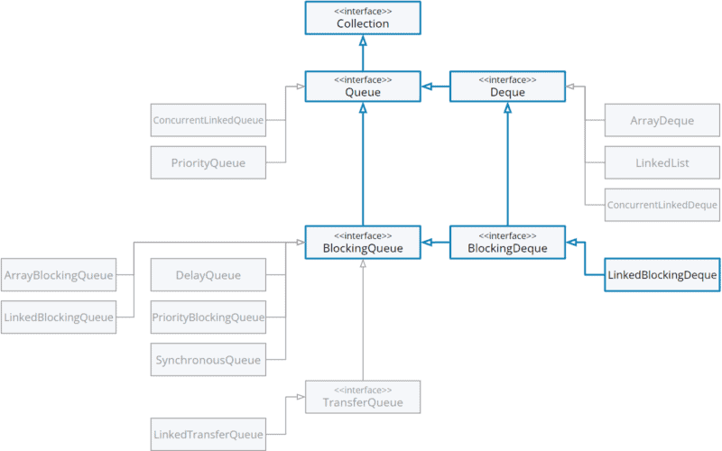


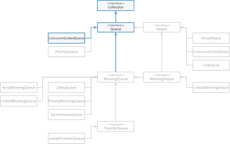


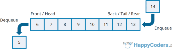


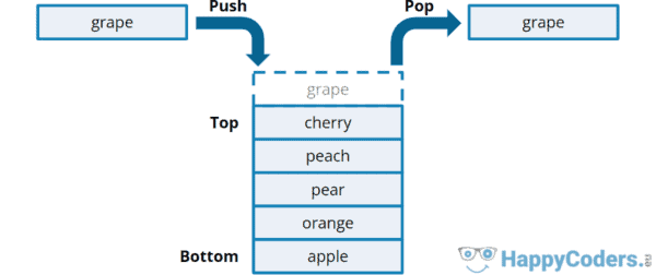


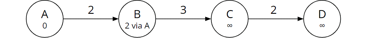


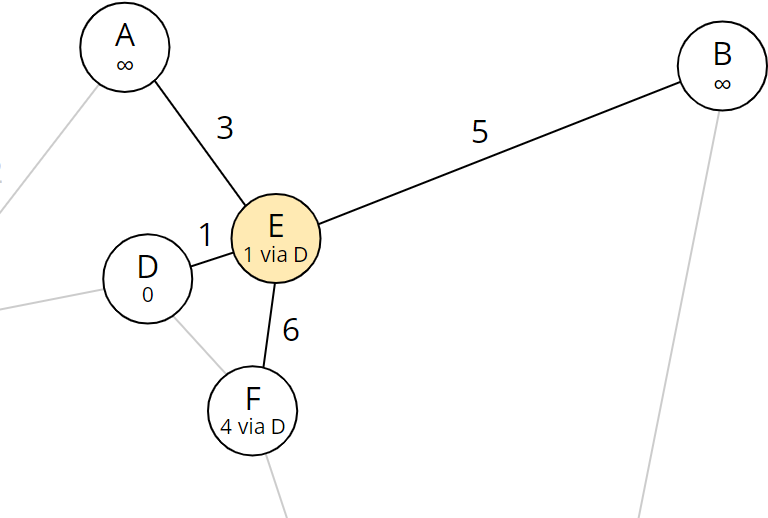


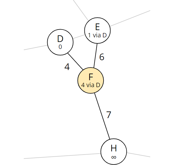


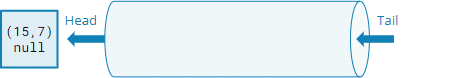
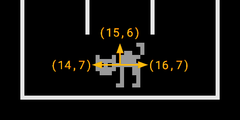


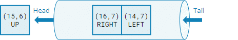
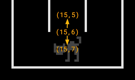
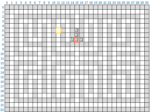


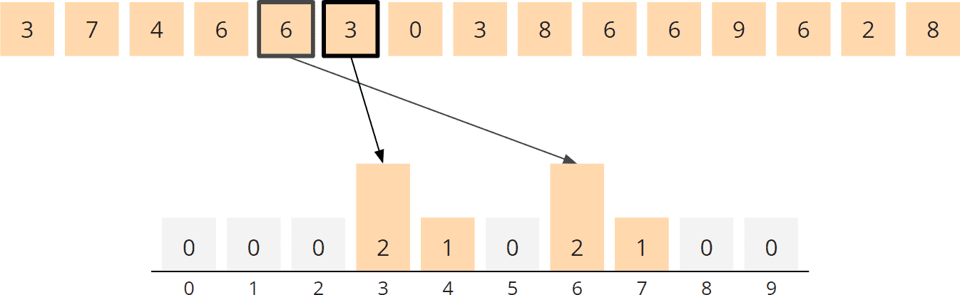


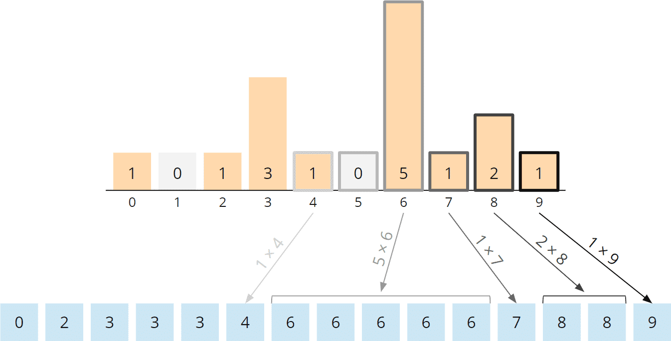


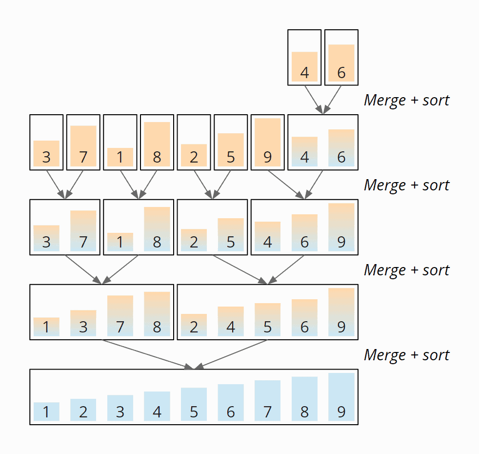


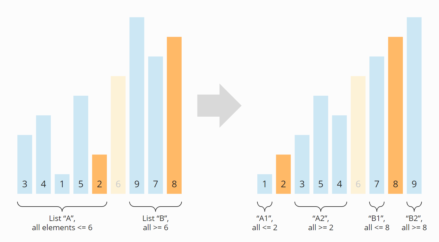


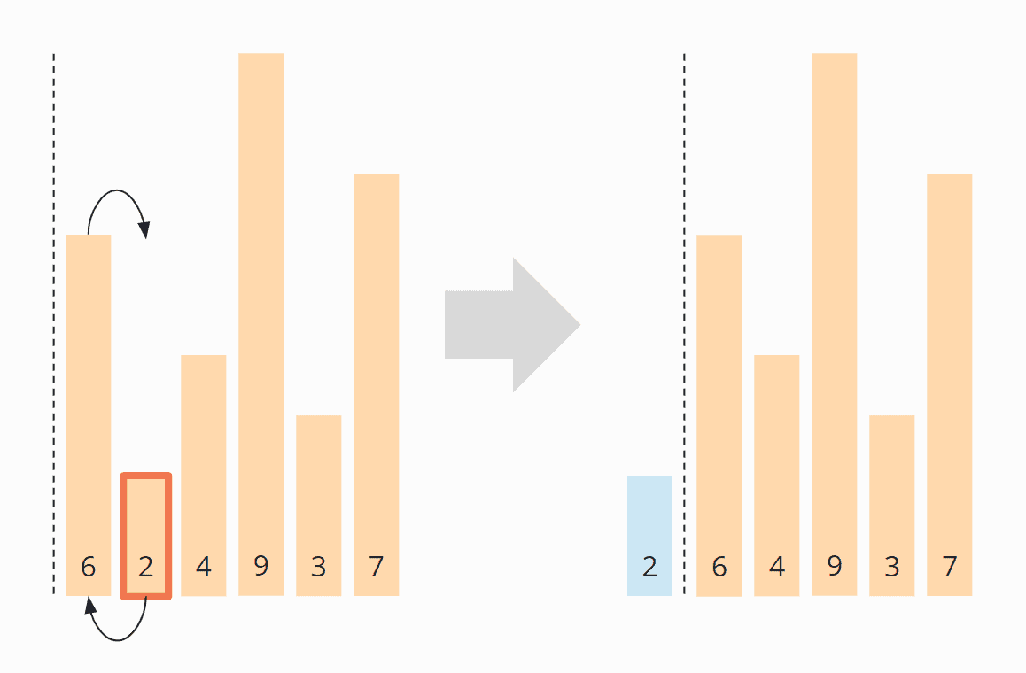


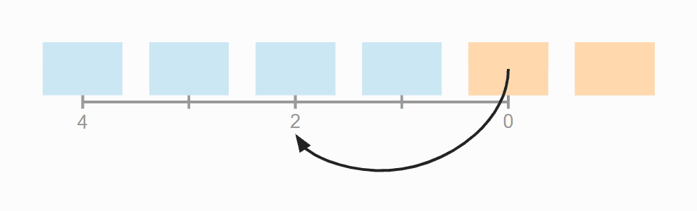
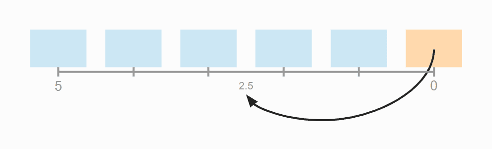


![Sorting in Java [Tutorial]](https://janice.happycoders.eu/wp-content/uploads/2020/06/sorting-in-java-feature-image.jpg)
![Sorting Algorithms [Ultimate Guide]](https://janice.happycoders.eu/wp-content/uploads/2020/06/sorting-algorithms-java-feature-image.jpg)


