Tag: Data structures/Trees

The red-black tree is a widely used concrete implementation of a self-balancing binary search tree. In the JDK, it is used in TreeMap, and since Java 8, it is also used for bucket collisions in HashMap. How does it work?

In this article, you will learn:

• What is a red-black tree?
• How do you insert elements into a red-black tree? How do you remove them?
• What are the rules for balancing a red-black tree?
• How to implement a red-black tree in Java?
• How to determine its time complexity?
• What distinguishes a red-black tree from other data structures?

You can find the source code for the article in this GitHub repository.

What Is a Red-Black Tree?

A red-black tree is a self-balancing binary search tree, that is, a binary search tree that automatically maintains some balance.

Each node is assigned a color (red or black). A set of rules specifies how these colors must be arranged (e.g., a red node may not have red children). This arrangement ensures that the tree maintains a certain balance.

After inserting and deleting nodes, quite complex algorithms are applied to check compliance with the rules – and, in case of deviations, to restore the prescribed properties by recoloring nodes and rotations.

NIL Nodes in Red-Black Trees

In the literature, red-black trees are depicted with and without so-called NIL nodes. A NIL node is a leaf that does not contain a value. NIL nodes become relevant for the algorithms later on, e.g., to determine colors of uncle or sibling nodes.

In Java, NIL nodes can be represented simply by null references; more on this later.

Red-Black Tree Example

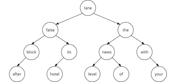
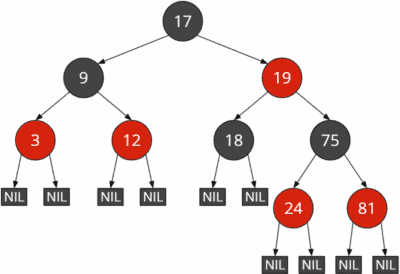
The following example shows two possible representations of a red-black tree. The first image shows the tree without (i.e., with implicit) NIL leaves; the second image shows the tree with explicit NIL leaves.

In the course of this tutorial, I will generally refrain from showing the NIL leaves. When explaining the insert and delete operations, I will show them sporadically if it facilitates understanding the respective algorithm.

Red-Black Tree Properties

The following rules enforce the red-black tree balance:

1. Each node is either red or black.
2. (The root is black.)
3. All NIL leaves are black.
4. A red node must not have red children.
5. All paths from a node to the leaves below contain the same number of black nodes.

Rule 2 is in parentheses because it does not affect the tree’s balance. If a child of a red root is also red, the root must be colored black according to rule 4. However, if a red root has only black children, there is no advantage in coloring the root black.

Therefore, rule 2 is often omitted in the literature.

When explaining the insert and delete operations and in the Java code, I will point out where there would be differences if we would also implement rule 2. So much in advance: The difference is only one line of code per operation :)

By the way, from rules 4 and 5 follows that a red node always has either two NIL leaves or two black child nodes with values. If it had one NIL leaf and one black child with value, then the paths through this child would have at least one more black node than the path to the NIL leaf, which would violate rule 5.

Height of a Red-Black Tree

We refer to the height of the red-black tree as the maximum number of nodes from the root to a NIL leaf, not including the root. The height of the red-black tree in the example above is 4:

From rules 3 and 4 follows:

The longest path from the root to a leaf (not counting the root) is at most twice as long as the shortest path from the root to a leaf.

That is easily explained:

Let’s assume that the shortest path has (in addition to the root) n black nodes and no red nodes. Then we could add another n red nodes before each black node without breaking rule 3 (which we could reword to: no two red nodes may follow each other).

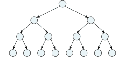
The following example shows the shortest possible path through a red-black tree of height four on the left and the longest possible path on the right:

The paths to the NIL leaves on the left have a length (excluding the root) of 2. The paths to the NIL leaves on the bottom right have a length of 4.

Black Height of a Red-Black Tree

Black height is the number of black nodes from a given node to its leaves. The black NIL leaves are counted, the start node is not.

The black height of the entire tree is the number of black nodes from the root (this is not counted) to the NIL leaves.

The black height of all red-black trees shown so far is 2.

Red-Black Tree Java Implementation

As a starting point for implementing the red-black tree in Java, I use the Java source code for the binary search tree from the second part of the binary tree series.

Nodes are represented by the Node class. For simplicity, we use int primitives as the node value.

To implement the red-black tree, besides the child nodes left and right, we need a reference to the parent node and the node’s color. We store the color in a boolean, defining red as false and black as true.

public class Node {
  int data;

  Node left;
  Node right;
  Node parent;

  boolean color;

  public Node(int data) {
    this.data = data;
  }
}Code language: Java (java)

We implement the red-black tree in the RedBlackTree class. This class extends the BaseBinaryTree class presented in the second part of the series (which essentially provides a getRoot() function).

We will add the operations (insert, search, delete) in the following sections, step by step.

But first, we have to define some helper functions.

Red Black Tree Rotation

Insertion and deletion work basically as described in the article about binary search trees.

After insertion and deletion, the red-black rules (see above) are reviewed. If they have been violated, they must be restored. That happens by recoloring nodes and by rotations.

The rotation works precisely like with AVL trees, which I described in the previous tutorial. I’ll show you the corresponding diagrams again here. You can find detailed explanations in the section “AVL tree rotation” of the article just mentioned.

Right Rotation

The following graphic shows a right rotation. The colors have no relation to those of the red-black tree. They are only used to track the node movements better.

The left node L becomes the new root; the root N becomes its right child. The right child LR of the pre-rotation left node L becomes the left child of the post-rotation right node N. The two white nodes LL and R do not change their relative position.

The Java code is slightly longer than in the AVL tree – for the following two reasons:

1. We also need to update the parent references of the nodes (in the AVL tree, we worked without parent references).
2. We need to update the references to and from the pre-rotation top node’s parent (N in the graphic). For the AVL tree, we did that indirectly by returning the new root of the rotated subtree and “hooking” the rotation into the recursive call of the insert and delete operations.

You can find the implementation of the right rotation in the source code starting at line 358:

private void rotateRight(Node node) {
  Node parent = node.parent;
  Node leftChild = node.left;

  node.left = leftChild.right;
  if (leftChild.right != null) {
    leftChild.right.parent = node;
  }

  leftChild.right = node;
  node.parent = leftChild;

  replaceParentsChild(parent, node, leftChild);
}Code language: Java (java)

The replaceParentsChild() method called at the end sets the parent-child relationship between the parent node of the former root node N of the rotated subtree and its new root node L. You can find it in the code starting at line 388:

private void replaceParentsChild(Node parent, Node oldChild, Node newChild) {
  if (parent == null) {
    root = newChild;
  } else if (parent.left == oldChild) {
    parent.left = newChild;
  } else if (parent.right == oldChild) {
    parent.right = newChild;
  } else {
    throw new IllegalStateException("Node is not a child of its parent");
  }

  if (newChild != null) {
    newChild.parent = parent;
  }
}Code language: Java (java)

Left Rotation

Left rotation works analogously: The right node R moves up to the top. The root N becomes the left child of R. The left child RL of the formerly right node R becomes the right child of the post-rotation left node N. L and RR do not change their relative position.

Here is the Java code for the left rotation (source code, starting at line 373):

private void rotateLeft(Node node) {
  Node parent = node.parent;
  Node rightChild = node.right;

  node.right = rightChild.left;
  if (rightChild.left != null) {
    rightChild.left.parent = node;
  }

  rightChild.left = node;
  node.parent = rightChild;

  replaceParentsChild(parent, node, rightChild);
}Code language: Java (java)

Red-Black Tree Operations

Like any binary tree, the red-black tree provides operations to find, insert, and delete nodes. We will go through these operations step by step in the following sections.

At this point, I would like to recommend the red-black tree simulator by David Galles. It allows you to animate any insert, delete and search operations graphically.

Red-Black Tree Search

The search works like in any binary search tree: We first compare the search key with the root. If the search key is smaller, we continue the search in the left subtree; if the search key is larger, we continue the search in the right subtree.

We repeat this until we either find the node we are looking for – or until we reach a NIL leaf (in Java code: a null reference). Reaching a NIL leaf would mean that the key we are looking for does not exist in the tree.

For a graphical representation of the search, see the example in the article about binary search trees.

For the red-black tree, we implement an iterative variant of the search. You can find it in the source code starting at line 14:

public Node searchNode(int key) {
  Node node = root;
  while (node != null) {
    if (key == node.data) {
      return node;
    } else if (key < node.data) {
      node = node.left;
    } else {
      node = node.right;
    }
  }

  return null;
}Code language: Java (java)

This code should be self-explanatory.

In the “Searching” section of the article mentioned above, you can also find a recursive version of the search.

Red-Black Tree Insertion

To insert a new node, we first proceed as described in the “binary search tree insertion” section of the corresponding article. I.e., we search for the insertion position from the root downwards and attach the new node to a leaf or half-leaf.

You can find the code in the RedBlackTree class, starting at line 29:

public void insertNode(int key) {
  Node node = root;
  Node parent = null;

  // Traverse the tree to the left or right depending on the key
  while (node != null) {
    parent = node;
    if (key < node.data) {
      node = node.left;
    } else if (key > node.data) {
      node = node.right;
    } else {
      throw new IllegalArgumentException("BST already contains a node with key " + key);
    }
  }

  // Insert new node
  Node newNode = new Node(key);
  newNode.color = RED;
  if (parent == null) {
    root = newNode;
  } else if (key < parent.data) {
    parent.left = newNode;
  } else {
    parent.right = newNode;
  }
  newNode.parent = parent;

  fixRedBlackPropertiesAfterInsert(newNode);
}
Code language: Java (java)

We initially color the new node red so that rule 5 is satisfied, i.e., all paths have the same number of black nodes after insertion.

However, if the parent node of the inserted node is also red, we have violated rule 4. We then have to repair the tree by recoloring and/or rotating it so that all rules are satisfied again. That is done in the fixRedBlackPropertiesAfterInsert() method, which is called in the last line of the insertNode() method.

During the repair, we have to deal with five different cases:

• Case 1: New node is the root
• Case 2: Parent node is red and the root
• Case 3: Parent and uncle nodes are red
• Case 4: Parent node is red, uncle node is black, inserted node is “inner grandchild”
• Case 5: Parent node is red, uncle node is black, inserted node is “outer grandchild”

The five cases are described below.

Case 1: New Node Is the Root

If the new node is the root, we don’t have to do anything else. Unless we work with rule 2 (“the root is always black”). In that case, we would have to color the root black.

Case 2: Parent Node Is Red and the Root

In this case, rule 4 (“no red-red!”) is violated. All we have to do now is to color the root black. That leads to rule 4 being complied with again.

And rule 5? Since the root is not counted in this rule, all paths still have one black node (the NIL leaves not displayed in the graphic). And if we would count the root, then all paths would now have two black nodes instead of one – that would also be allowed.

If we work with rule 2 (“the root is always black”), we have already colored the root black in case 1, and case 2 can no longer occur.

Case 3: Parent and Uncle Nodes Are Red

We use the term “uncle node” to refer to the sibling of the parent node; that is, the second child of the grandparent node next to the parent node. The following graphic should make this understandable: Inserted was the 81; its parent is the 75, the grandparent is the 19, and the uncle is the 18.

Both the parent and the uncle are red. In this case, we do the following:

We recolor parent and uncle nodes (18 and 75 in the example) black and the grandparent (19) red. Thus rule 4 (“no red-red!”) is satisfied again at the inserted node. The number of black nodes per path does not change (in the example, it remains at 2).

However, there could now be two red nodes in a row at the grandparent node – namely, if the great-grandparent node (17 in the example) were also red. In this case, we would have to make further repairs. We would do this by calling the repair function recursively on the grandparent node.

Case 4: Parent Node Is Red, Uncle Node Is Black, Inserted Node Is “Inner Grandchild”

I must first explain this case: “inner grandchild” means that the path from the grandparent node to the inserted node forms a triangle, as shown in the following graphic using 19, 75, and 24. In this example, you can see that a NIL leaf is also considered a black uncle (according to rule 3).

(For the sake of clarity, I have not drawn the two NIL leaves of the 9 and the 24, as well as the right NIL leaf of the 75.)

In this case, we first rotate at the parent node in the opposite direction of the inserted node.

What does that mean?

If the inserted node is the left child of its parent node, we rotate to the right at the parent node. If the inserted node is the right child, we rotate to the left.

In the example, the inserted node (the 24) is a left child, so we rotate to the right at the parent node (75 in the example):

Second, we rotate at the grandparent node in the opposite direction to the previous rotation. In the example, we rotate left around the 19:

Finally, we color the node we just inserted (the 24 in the example) black and the original grandparent (the 19 in the example) red:

Since there is now a black node at the top of the last rotated subtree, there cannot be a violation of rule 4 (“no red-red!”) at that position.

Also, recoloring the original grandparent (19) red cannot violate rule 4. Its left child is the uncle, which is black by definition of this case. And the right child, as a result of the second rotation, is the left child of the inserted node, thus a black NIL leaf.

The inserted red 75 has two NIL leaves as children, so there is no violation of rule 4 here either.

The repair is now complete; a recursive call of the repair function is not necessary.

Case 5: Parent Node Is Red, Uncle Node Is Black, Inserted Node Is “Outer Grandchild”

“Outer grandchild” means that the path from grandparent to inserted node forms a line, such as the 19, 75, and 81 in the following example:

In this case, we rotate at the grandparent (19 in the example) in the opposite direction of the parent and inserted node (after all, both go in the same direction in this case). In the example, the parent and inserted nodes are both right children, so we rotate left at the grandparent:

Then we recolor the former parent (75 in the example) black and the former grandparent (19) red:

As at the end of case 4, we have a black node at the top of the rotation, so there can be no violation of rule 4 (“no red-red!”) there.

The left child of the 19 is the original uncle after rotation, so it is black by case definition. The right child of the 19 is the original left child of the parent node (75), which must also be a black NIL leaf; otherwise, the right place where we inserted the 81 would not have been free (because a red node always has either two black children with value or two black NIL children).

The red 81 is the inserted node and, therefore, also has two black NIL leaves.

At this point, we’ve completed the repair of the red-black tree.

If you have paid close attention, you will notice that case 5 corresponds precisely to the second rotation from case 4. In the code, this will be shown by the fact that only the first rotation is implemented for case 4, and then the program jumps to the code for case 5.

Implementation of the Post-Insertion Repair Method

You can find the complete repair function in RedBlackTree starting at line 64. I have marked cases 1 to 5 by comments. Cases 4 and 5 are split into 4a/4b and 5a/5b depending on whether the parent node is left (4a/5a) or right child (4b/5b) of the grandparent node.

private void fixRedBlackPropertiesAfterInsert(Node node) {
  Node parent = node.parent;

  // Case 1: Parent is null, we've reached the root, the end of the recursion
  if (parent == null) {
    // Uncomment the following line if you want to enforce black roots (rule 2):
    // node.color = BLACK;
    return;
  }

  // Parent is black --> nothing to do
  if (parent.color == BLACK) {
    return;
  }

  // From here on, parent is red
  Node grandparent = parent.parent;

  // Case 2:
  // Not having a grandparent means that parent is the root. If we enforce black roots
  // (rule 2), grandparent will never be null, and the following if-then block can be
  // removed.
  if (grandparent == null) {
    // As this method is only called on red nodes (either on newly inserted ones - or -
    // recursively on red grandparents), all we have to do is to recolor the root black.
    parent.color = BLACK;
    return;
  }

  // Get the uncle (may be null/nil, in which case its color is BLACK)
  Node uncle = getUncle(parent);

  // Case 3: Uncle is red -> recolor parent, grandparent and uncle
  if (uncle != null && uncle.color == RED) {
    parent.color = BLACK;
    grandparent.color = RED;
    uncle.color = BLACK;

    // Call recursively for grandparent, which is now red.
    // It might be root or have a red parent, in which case we need to fix more...
    fixRedBlackPropertiesAfterInsert(grandparent);
  }

  // Parent is left child of grandparent
  else if (parent == grandparent.left) {
    // Case 4a: Uncle is black and node is left->right "inner child" of its grandparent
    if (node == parent.right) {
      rotateLeft(parent);

      // Let "parent" point to the new root node of the rotated sub-tree.
      // It will be recolored in the next step, which we're going to fall-through to.
      parent = node;
    }

    // Case 5a: Uncle is black and node is left->left "outer child" of its grandparent
    rotateRight(grandparent);

    // Recolor original parent and grandparent
    parent.color = BLACK;
    grandparent.color = RED;
  }

  // Parent is right child of grandparent
  else {
    // Case 4b: Uncle is black and node is right->left "inner child" of its grandparent
    if (node == parent.left) {
      rotateRight(parent);

      // Let "parent" point to the new root node of the rotated sub-tree.
      // It will be recolored in the next step, which we're going to fall-through to.
      parent = node;
    }

    // Case 5b: Uncle is black and node is right->right "outer child" of its grandparent
    rotateLeft(grandparent);

    // Recolor original parent and grandparent
    parent.color = BLACK;
    grandparent.color = RED;
  }
}Code language: Java (java)

You will find the helper function getUncle() starting at line 152:

private Node getUncle(Node parent) {
  Node grandparent = parent.parent;
  if (grandparent.left == parent) {
    return grandparent.right;
  } else if (grandparent.right == parent) {
    return grandparent.left;
  } else {
    throw new IllegalStateException("Parent is not a child of its grandparent");
  }
}Code language: Java (java)

Implementation Notes

Unlike the AVL tree, we cannot easily hook the repair function of the red-black tree into the existing recursion from BinarySearchTreeRecursive. That is because we need to rotate not only at the node under which we inserted the new node but also at the grandparent if necessary (cases 3 and 4).

You will find numerous alternative implementations in the literature. These are sometimes minimally more performant than the way presented here since they combine multiple steps. That doesn’t change the order of magnitude of the performance, but it can gain a few percent. It was important for me to implement the algorithm in a comprehensible way. The more performant algorithms are always more complex, too.

I implemented the iterative insertion in two steps – search first, then insertion – unlike BinarySearchTreeIterative, where I combined the two. That makes reading the code a bit easier but requires an additional “if (key < parent.data)” check to determine whether the new node needs to be inserted as a left or right child under its parent.

Red-Black Tree Deletion

If you have just finished reading the chapter on inserting, you might want to take a short break. After all, deleting is even more complex.

First, we proceed as described in the “Binary Search Tree Deletion” section of the article on binary search trees in general.

Here is a summary:

1. If the node to be deleted has no children, we simply remove it.
2. If the node to be deleted has one child, we remove the node and let its single child move up to its position.
3. If the node to be deleted has two children, we copy the content (not the color!) of the in-order successor of the right child into the node to be deleted and then delete the in-order successor according to rule 1 or 2 (the in-order successor has at most one child by definition).

After that, we need to check the rules of the tree and repair it if necessary. To do this, we need to remember the deleted node’s color and which node we have moved up.

• If the deleted node is red, we cannot have violated any rule: Neither can it result in two consecutive red nodes (rule 4), nor does it change the number of black nodes on any path (rule 5).
• However, if the deleted node is black, we are guaranteed to have violated rule 5 (unless the tree contained nothing but a black root), and rule 4 may also have been violated – namely if both parent nodes and the moved-up child of the deleted node were red.

First, here is the code for the actual deletion of a node (class RedBlackTree, line 163). Underneath the code, I will explain its parts:

public void deleteNode(int key) {
  Node node = root;

  // Find the node to be deleted
  while (node != null && node.data != key) {
    // Traverse the tree to the left or right depending on the key
    if (key < node.data) {
      node = node.left;
    } else {
      node = node.right;
    }
  }

  // Node not found?
  if (node == null) {
    return;
  }

  // At this point, "node" is the node to be deleted

  // In this variable, we'll store the node at which we're going to start to fix the R-B
  // properties after deleting a node.
  Node movedUpNode;
  boolean deletedNodeColor;

  // Node has zero or one child
  if (node.left == null || node.right == null) {
    movedUpNode = deleteNodeWithZeroOrOneChild(node);
    deletedNodeColor = node.color;
  }

  // Node has two children
  else {
    // Find minimum node of right subtree ("inorder successor" of current node)
    Node inOrderSuccessor = findMinimum(node.right);

    // Copy inorder successor's data to current node (keep its color!)
    node.data = inOrderSuccessor.data;

    // Delete inorder successor just as we would delete a node with 0 or 1 child
    movedUpNode = deleteNodeWithZeroOrOneChild(inOrderSuccessor);
    deletedNodeColor = inOrderSuccessor.color;
  }

  if (deletedNodeColor == BLACK) {
    fixRedBlackPropertiesAfterDelete(movedUpNode);

    // Remove the temporary NIL node
    if (movedUpNode.getClass() == NilNode.class) {
      replaceParentsChild(movedUpNode.parent, movedUpNode, null);
    }
  }
}Code language: Java (java)

The first lines of code search for the node to be deleted; the method terminates if that node can’t be found.

How to proceed depends on the number of children nodes to be deleted.

Deleting a Node With Zero or One Child

If the deleted node has at most one child, we call the method deleteNodeWithZeroOrOneChild(). You can find it in the source code starting at line 221:

private Node deleteNodeWithZeroOrOneChild(Node node) {
  // Node has ONLY a left child --> replace by its left child
  if (node.left != null) {
    replaceParentsChild(node.parent, node, node.left);
    return node.left; // moved-up node
  }

  // Node has ONLY a right child --> replace by its right child
  else if (node.right != null) {
    replaceParentsChild(node.parent, node, node.right);
    return node.right; // moved-up node
  }

  // Node has no children -->
  // * node is red --> just remove it
  // * node is black --> replace it by a temporary NIL node (needed to fix the R-B rules)
  else {
    Node newChild = node.color == BLACK ? new NilNode() : null;
    replaceParentsChild(node.parent, node, newChild);
    return newChild;
  }
}Code language: Java (java)

I have already introduced you to the replaceParentsChild() method (which is called several times here) in the rotation.

The case where the deleted node is black and has no children is a special case. That is dealt with in the last else block:

We have seen above that deleting a black node results in the number of black nodes no longer being the same on all paths. That is, we will have to repair the tree. The tree repair always starts (as you will see shortly) at the moved-up node.

If the deleted node has no children, one of its NIL leaves virtually moves up to its position. To be able to navigate from this NIL leaf to its parent node later, we need a special placeholder. I’ve implemented one in the class NilNode, which you can find in the source code starting at line 349:

private static class NilNode extends Node {
  private NilNode() {
    super(0);
    this.color = BLACK;
  }
}Code language: Java (java)

Finally, the deleteNodeWithZeroOrOneChild() method returns the moved-up node that the calling deleteNode() method stores in the movedUpNode variable.

Deleting a Node With Two Children

If the node to be deleted has two children, we first use the findMinimum() method (line 244) to find the in-order successor of the subtree that starts at the right child:

private Node findMinimum(Node node) {
  while (node.left != null) {
    node = node.left;
  }
  return node;
}Code language: Java (java)

We then copy the data of the in-order successor into the node to be deleted and call the deleteNodeWithZeroOrOneChild() method introduced above to remove the in-order successor from the tree. Again, we remember the moved-up node in movedUpNode.

Repairing the Tree

Here is once more the last if-block of the deleteNode() method:

if (deletedNodeColor == BLACK) {
  fixRedBlackPropertiesAfterDelete(movedUpNode);

  // Remove the temporary NIL node
  if (movedUpNode.getClass() == NilNode.class) {
    replaceParentsChild(movedUpNode.parent, movedUpNode, null);
  }
}Code language: Java (java)

As stated above, deleting a red node does not violate any rules. If, however, the deleted node is black, we call the repair method fixRedBlackPropertiesAfterDelete().

If any, we’ve needed the temporary NilNode placeholder created in deleteNodeWithZeroOrOneChild() only for calling the repair function. We can therefore remove it afterward.

When deleting, we have to consider one more case than when inserting. In contrast to the insertion, the color of the uncle is not relevant here but that of the deleted node’s sibling.

• Case 1: Deleted node is the root
• Case 2: Sibling is red
• Case 3: Sibling is black and has two black children, parent is red
• Case 4: Sibling is black and has two black children, parent is black
• Case 5: Sibling is black and has at least one red child, “outer nephew” is black
• Case 6: Sibling is black and has at least one red child, “outer nephew” is red

The following sections describe the six cases in detail:

Case 1: Deleted Node Is the Root

If we removed the root, another node moved up to its position. That could only happen if the root had zero or only one child. If the root had had two children, it would have been the in-order successor that would have been removed in the end and not the root node.

If the root had no child, the new root is a black NIL node. Thus the tree is empty and valid:

If the root had one child, then this had to be red and have no other children.

Explanation: If the red child had another red child, rule 4 (“no red-red!”) would have been violated. If the red child had a black child, then the paths through the red node would have at least one more black node than the NIL subtree of the root, and thus rule 5 would have been violated.

Thus, the tree consists of only one red root and is therefore also valid.

Should we work with rule 2 (“the root is always black”), we would now recolor the root.

Case 2: Sibling Is Red

For all other cases, we first check the color of the sibling. That is the second child of the parent of the deleted node. In the following example, we delete the 9; its sibling is the red 19:

In this case, we first color the sibling black and the parent red:

That obviously violated rule 5: The paths in the right subtree of the parent each have two more black nodes than those in the left subtree. We fix this by rotating around the parent in the direction of the deleted node.

In the example, we have deleted the left node of the parent node – we, therefore, perform a left rotation:

Now we have two black nodes on the right path and two on the path to the 18. However, we have only one black node on the path to the left NIL leaf of 17 (remember: the root does not count, the NIL nodes do – even the ones not drawn in the graphic).

We look at the new sibling of the deleted node (18 in the example). That new sibling is now definitely black because it is an original child of the red sibling from the beginning of the case.

Also, the new sibling has black children. Therefore, we color the sibling (the 18) red and the parent (the 17) black:

Now all paths have two black nodes; we have a valid red-black tree again.

Case 2 ‒ Fall-Through

In fact, I have anticipated something in this last step. Namely, we have executed the rules of case 3 (that’s why the image subtitle is in parentheses).

In this last step of case 2, we always have a black sibling. The fact that the black sibling had two black children, as required for case 3, was a coincidence. In fact, at the end of case 2, any of the cases 3 to 6 can occur and must be treated according to the following sections.

Case 3: Sibling Is Black and Has Two Black Children, Parent Is Red

In the following example, we delete the 75 and let one of its black NIL leaves move up.

(Again, as a reminder: I only show NIL nodes in the graphics when they are relevant for understanding.)

The deletion violates rule 5: In the rightmost path, we now have one black node less than in all others.

The sibling (the 18 in the example) is black and has two black children (the NIL leaves not shown). The parent (the 19) is red. In this case, we repair the tree as follows:

We recolor the sibling (the 18) red and the parent (the 19) black:

Thus we have a valid red-black tree again. The number of black nodes is the same on all paths (as required by rule 5). And since the sibling has only black children, coloring it red cannot violate rule 4 (“no red-red!”).

Case 4: Sibling Is Black and Has Two Black Children, Parent Is Black

In the following example, we delete the 18:

This leads (just like in case 3) to a violation of rule 5: On the path to the deleted node, we now have one black node less than on all other paths.

In contrast to case 3, in this case, the parent node of the deleted node is black. We first color the sibling red:

That means that the black height in the subtree that starts at the parent node is again uniform (2). In the left subtree, however, it is one higher (3). Rule 5 is therefore still violated.

Case 4 ‒ Recursion

We solve this problem by pretending that we deleted a black node between nodes 17 and 19 (which would have had the same effect). Accordingly, we call the repair function recursively on the parent node, i.e., the 19 (which would have been the moved-up node in this case).

The 19 has a black sibling (the 9) with two black children (3 and 12) and a red parent (17). Accordingly, we are now back to case 3.

We solve case 3 by coloring the parent black and the sibling red:

The black height is now two on all paths, so our red-black tree is valid again.

Case 5: Sibling is black and has at least one red child, “outer nephew” is black

In this example, we delete the 18:

As a result, we again violated rule 5 since the subtree starting at the sibling now has a black height greater by one.

We examine the “outer nephew” of the deleted node. “Outer nephew” means the child of the sibling that is opposite the deleted node. In the example, this is the right (and by definition black) NIL leaf under the 75.

In the following graphic, you can see that parent, sibling and nephew together form a line (in the example: 19, 75, and its right NIL child).

We start the repair by coloring the inner nephew (the 24 in the example) black and the sibling (the 75) red:

Then we perform a rotation at the sibling node in the opposite direction of the deleted node. In the example, we’ve deleted the parent’s left child, so we perform a right rotation at the sibling (the 75):

We are doing some recoloring again:

• We recolor the sibling in the color of its parent (in the example, the 24 red).
• Then we recolor the parent (the 19) and the outer nephew of the deleted node, i.e., the right child of the new sibling (the 75 in the example) black:

Finally, we perform a rotation on the parent node in the direction of the deleted node. In the example, the deleted node was a left child, so we perform a left rotation accordingly (at 19 in the example):

This last step restores compliance with all red-black rules. There are no two consecutive red nodes, and the number of black nodes is uniformly two on all paths. We’ve thus completed the repair of the tree.

Case 6: Sibling is black and has at least one red child, “outer nephew” is red

In the last example, which is very similar to case 5, we also delete the 18:

As a result, as in case 5, we violated rule 5 because the path to the deleted node now contains one less black node.

In case 6, unlike case 5, the outer nephew (81 in the example) is red and not black.

We first recolor the sibling in the parent’s color (in the example, the 75 red). Then we recolor the parent (the 19 in the example) and the outer nephew (the 81) black:

Second, we perform a rotation at the parent node in the direction of the deleted node. In the example, we’ve deleted a left child; accordingly, we perform a left rotation around the 19:

This rotation restores the red-black rules. No two red nodes follow each other, and the number of black nodes is the same on all paths (namely 2).

The rules in this last case are similar to the final two steps of case 5. In the source code, you will see that for case 5, only its first two steps are implemented, and the program then goes to case 6 to execute the last two steps.

With this, we have studied all six cases. Let’s move on to the implementation of the repair function in Java.

Implementation of the Post-Deletion Repair Method

You can find the fixRedBlackPropertiesAfterDelete() method in the source code starting at line 252. I have marked cases 1 to 6 with comments.

private void fixRedBlackPropertiesAfterDelete(Node node) {
  // Case 1: Examined node is root, end of recursion
  if (node == root) {
    // Uncomment the following line if you want to enforce black roots (rule 2):
    // node.color = BLACK;
    return;
  }

  Node sibling = getSibling(node);

  // Case 2: Red sibling
  if (sibling.color == RED) {
    handleRedSibling(node, sibling);
    sibling = getSibling(node); // Get new sibling for fall-through to cases 3-6
  }

  // Cases 3+4: Black sibling with two black children
  if (isBlack(sibling.left) && isBlack(sibling.right)) {
    sibling.color = RED;

    // Case 3: Black sibling with two black children + red parent
    if (node.parent.color == RED) {
      node.parent.color = BLACK;
    }

    // Case 4: Black sibling with two black children + black parent
    else {
      fixRedBlackPropertiesAfterDelete(node.parent);
    }
  }

  // Case 5+6: Black sibling with at least one red child
  else {
    handleBlackSiblingWithAtLeastOneRedChild(node, sibling);
  }
}Code language: Java (java)

You will find the helper methods getSibling() and isBlack() starting at line 334:

private Node getSibling(Node node) {
  Node parent = node.parent;
  if (node == parent.left) {
    return parent.right;
  } else if (node == parent.right) {
    return parent.left;
  } else {
    throw new IllegalStateException("Parent is not a child of its grandparent");
  }
}

private boolean isBlack(Node node) {
  return node == null || node.color == BLACK;
}Code language: Java (java)

Handling a red sibling (case 2) starts at line 289:

private void handleRedSibling(Node node, Node sibling) {
  // Recolor...
  sibling.color = BLACK;
  node.parent.color = RED;

  // ... and rotate
  if (node == node.parent.left) {
    rotateLeft(node.parent);
  } else {
    rotateRight(node.parent);
  }
}Code language: Java (java)

You can find the implementation for a black sibling knot with at least one red child (cases 5 and 6) starting at line 302:

private void handleBlackSiblingWithAtLeastOneRedChild(Node node, Node sibling) {
  boolean nodeIsLeftChild = node == node.parent.left;

  // Case 5: Black sibling with at least one red child + "outer nephew" is black
  // --> Recolor sibling and its child, and rotate around sibling
  if (nodeIsLeftChild && isBlack(sibling.right)) {
    sibling.left.color = BLACK;
    sibling.color = RED;
    rotateRight(sibling);
    sibling = node.parent.right;
  } else if (!nodeIsLeftChild && isBlack(sibling.left)) {
    sibling.right.color = BLACK;
    sibling.color = RED;
    rotateLeft(sibling);
    sibling = node.parent.left;
  }

  // Fall-through to case 6...

  // Case 6: Black sibling with at least one red child + "outer nephew" is red
  // --> Recolor sibling + parent + sibling's child, and rotate around parent
  sibling.color = node.parent.color;
  node.parent.color = BLACK;
  if (nodeIsLeftChild) {
    sibling.right.color = BLACK;
    rotateLeft(node.parent);
  } else {
    sibling.left.color = BLACK;
    rotateRight(node.parent);
  }
}Code language: Java (java)

Just as for inserting, you will find numerous alternative approaches for deleting in the literature. I have tried to structure the code so that you can follow the code flow as well as possible.

Traversing the Red-Black Tree

Like any binary tree, we can traverse the red-black tree in pre-order, post-order, in-order, reverse-in-order, and level-order. In the “Binary Tree Traversal” section of the introductory article on binary trees, I have described traversal in detail.

In that section, you will also find the corresponding Java source code, implemented in the classes DepthFirstTraversal, DepthFirstTraversalIterative, and DepthFirstTraversalRecursive.

The traversal methods work on the BinaryTree interface. Since RedBlackTree also implements this interface, we can easily apply the traversal methods to it as well.

Red-Black Tree Time Complexity

For an introduction to the topic of time complexity and O-notation, see this article.

We can determine the cost of searching, inserting, and deleting a node in the binary tree as follows:

Search Time

We follow a path from the root to the searched node (or to a NIL leaf). At each level, we perform a comparison. The effort for the comparison is constant.

The search cost is thus proportional to the tree height.

We denote by n the number of tree nodes. In the “Height of a Red-Black Tree” section, we have recognized that the longest path is at most twice as long as the shortest path. It follows that the height of the tree is bounded by O(log n).

A formal proof is beyond the scope of this article. You can read the proof on Wikipedia.

Thus, the time complexity for finding a node in a red-black tree is: O(log n)

Insertion Time

When inserting, we first perform a search. We have just determined the search cost as O(log n).

Next, we insert a node. The cost of this is constant regardless of the tree size, so O(1).

Then we check the red-black rules and restore them if necessary. We do this starting at the inserted node and ascending to the root. At each level, we perform one or more of the following operations:

• Checking the color of the parent node
• Determination of the uncle node and checking its color
• Recoloring one up to three nodes
• Performing one or two rotations

Each of these operations has constant time, O(1), in itself. The total time for checking and repairing the tree is therefore also proportional to its height.

So the time complexity for inserting into a red-black tree is also: O(log n)

Deletion Time

Just as with insertion, we first search for the node to be deleted in time O(log n).

Also, the deletion cost is independent of the tree size, so it is constant O(1).

For checking the rules and repairing the tree, one or more of the following operations occur – at most once per level:

• Checking the color of the deleted node
• Determining the sibling and examining its color
• Checking the colors of the sibling’s children
• Recoloring the parent node
• Recoloring the sibling node and one of its children
• Performing one or two rotations

These operations also all have a constant complexity in themselves. Thus, the total effort for checking and restoring the rules after deleting a node is also proportional to the tree height.

So the time complexity for deleting from a red-black tree is also: O(log n)

Red-Black Tree Compared With Other Data Structures

The following sections describe the differences and the advantages and disadvantages of the red-black tree compared to alternative data structures.

Red-Black Tree vs. AVL Tree

The red-black tree, as well as the AVL tree, are self-balancing binary search trees.

In the red-black tree, the longest path to the root is at most twice as long as the shortest path to the root. On the other hand, in the AVL tree, the depth of no two subtrees differs by more than 1.

In the red-black tree, balance is maintained by the node colors, a set of rules, and by rotating and recoloring nodes. In the AVL tree, the heights of the subtrees are compared, and rotations are performed when necessary.

These differences in the characteristics of the two types of trees lead to the following differences in performance and memory requirements:

• Due to the more even balancing of the AVL tree, search in an AVL tree is usually faster. In terms of magnitude, however, both are in the range O(log n).
• For insertion and deletion, the time complexity in both trees is O(log n). In a direct comparison, however, the red-black tree is faster because it rebalances less frequently.
• Both trees require additional memory: the AVL tree one byte per node for the height of the subtree starting at a node; the red-black tree one bit per node for the color information. This rarely makes a difference in practice since a single bit usually occupies at least one byte.

If you expect many insert/delete operations, then you should use a red-black tree. If, on the other hand, you expect more search operations, then you should choose the AVL tree.

Red-Black Tree vs. Binary Search Tree

The red-black tree is a concrete implementation of a self-balancing binary search tree. So every red-black tree is also a binary search tree.

There are also other types of binary search trees, such as the AVL tree mentioned above – or trivial non-balanced implementations. Thus, not every binary search tree is also a red-black tree.

Summary

This tutorial taught you what a red-black tree is, which rules govern it and how these rules are evaluated and restored if necessary after inserting and deleting nodes. I also introduced you to a Java implementation that is as easy to understand as possible.

The JDK uses red-black trees in TreeMap (here is the source code on GitHub) and in bucket collisions in HashMap (here is the source code).

With this, I conclude the tutorial series on binary trees.

If I could help you better understand binary trees in general, binary search trees, AVL trees, and – in this article – red-black trees, I’m happy about a comment.

An AVL tree is a concrete implementation of a self-balancing binary search tree. It was developed in 1962 by Soviet computer scientists Georgi Maximovich Adelson-Velsky and Yevgeny Mikhailovich Landis and named after their initials.

In this article, you’ll learn:

• What is an AVL tree?
• How to calculate the balance factor in an AVL tree?
• What is AVL tree rotation, and how does it work?
• How to insert elements, and how to delete them?
• How to implement an AVL tree in Java?
• What is the time complexity of the AVL tree operations?
• How does the AVL tree differ from the red-black tree?

You can find the source code for the article in this GitHub repository.

What Is an AVL Tree?

An AVL tree is a balanced binary search tree – that is, a binary search tree in which the heights of the left and right subtrees of each node differ by at most one.

After each insert and delete operation, this invariant is verified, and the balance is restored by AVL rotation if necessary.

Height of an AVL Tree

The height of a (sub) tree indicates how far the root is from the lowest node. Therefore, a (sub) tree that consists of only a root node has a height of 0.

AVL Tree Balance Factor

The balance factor “BF” of a node denotes the difference of the heights “H” of the right and left subtree (“node.right” and “node.left”):

BF(node) = H(node.right) – H(node.left)

The height of a non-existent subtree is -1 (one less than the height of a subtree consisting of only one node).

There are three cases:

• If the balance factor is < 0, the node is said to be left-heavy.
• If the balance factor is > 0, the node is said to be right-heavy.
• A balance factor of 0 represents a balanced node.

In an AVL tree, the balance factor at each node is -1, 0, or 1.

AVL Tree Example

The following example shows an AVL tree with height and balance factor specified at each node:

Nodes 2 and 7 in this example are right-heavy, node 4 is left-heavy. All other nodes are balanced.

The following tree, however, is not an AVL tree since the AVL criterion (-1 ≤ BF ≤ 1) is not fulfilled at node 4. Its left subtree has a height of 1, and the right, empty subtree has a height of -1. The difference between them is -2.

AVL Tree Implementation in Java

To implement the AVL tree in Java, we use the Java source code for the binary search tree from the previous tutorial in the binary tree series.

Nodes are represented by the Node class. For the node’s data field, we use int primitives for simplicity. In height, we store the height of the subtree whose root is this node.

public class Node {
  int data;
  Node left;
  Node right;

  int height;

  public Node(int data) {
    this.data = data;
  }
}Code language: GAUSS (gauss)

The AVL tree is implemented by the AvlTree class. It extends the BinarySearchTreeRecursive class introduced in the previous part. We will reuse much of its functionality.

For balancing the AVL tree, we need the following three additional methods:

• height() returns the height of a subtree stored in node.height ‒ or -1 for an empty subtree.
• updateHeight() sets node.height to the maximum height of the children plus 1.
• balanceFactor() calculates a node’s balance factor.

public class AvlTree extends BinarySearchTreeRecursive {

  private int height(Node node) {
    return node != null ? node.height : -1;
  }

  private void updateHeight(Node node) {
    int leftChildHeight = height(node.left);
    int rightChildHeight = height(node.right);
    node.height = max(leftChildHeight, rightChildHeight) + 1;
  }

  private int balanceFactor(Node node) {
    return height(node.right) - height(node.left);
  }

  // ...
}Code language: Java (java)

We will extend the code step by step in the following sections.

AVL Tree Rotation

Inserting into and deleting from an AVL tree works basically as described in the article about binary search trees.

If the AVL invariant is no longer fulfilled after an insert or delete operation, we must rebalance the tree. We will do that by so-called rotations.

We distinguish between right and left rotation.

Right Rotation

The following image shows a right rotation. The (sub) tree shown contains the following nodes:

• N: the node where an imbalance was detected
• L: the left child node of N
• LL: the left child node of L
• LR: the right child node of L
• R: the right child node of N

Under each letter, I have given an example node value in parentheses. This clearly shows that the following in-order sequence applies before the rotation:

LL (1) < L (2) < LR (3) < N (4) < R (5)

During rotation, node L moves to the root, and the previous root N becomes the right child of L. The previous right child of L, LR becomes the new left child of N. The two remaining nodes, LL and R remain unchanged relative to their parent node.

The example values in parentheses show clearly that the rotation has not changed the nodes’ in-order sequence.

The Java code for the right rotation is straightforward (class AvlTree, starting at line 71).

private Node rotateRight(Node node) {
  Node leftChild = node.left;

  node.left = leftChild.right;
  leftChild.right = node;

  updateHeight(node);
  updateHeight(leftChild);

  return leftChild;
}Code language: Java (java)

We memorize the left child leftChild (L in the image) of node (N in the image), replace the left child of node with the right child of the left child leftChild.right (LR in the image) and then set node as the new right child of the left child.

Then we update the heights of the subtrees in the order shown. I have already described the updateHeight() method in the “AVL Tree Implementation in Java” section.

The return value of the method is the new root node leftChild (L in the image).

Left Rotation

Left rotation works similarly:

Node R becomes the root; the previous root N becomes the left child of R. The previous left child of R, RL becomes the new right child of N. The relative positions of nodes RR and L do not change.

Also during left rotation, the in-order sequence of the nodes (L < N < RL < R < RR) is preserved.

The Java code looks as follows (class AvlTree, from line 83):

private Node rotateLeft(Node node) {
  Node rightChild = node.right;

  node.right = rightChild.left;
  rightChild.left = node;

  updateHeight(node);
  updateHeight(rightChild);

  return rightChild;
}Code language: Java (java)

AVL Tree Balancing

After insertion into or deletion from the AVL tree, we calculate the height and balance factor from the inserted or deleted node upwards to the root.

If, at a node, we determine that the AVL invariant is no longer satisfied (i.e., the balance factor is less than -1 or greater than +1), we must rebalance. We differentiate four cases:

• Balancing a left-heavy node:
  • Right rotation
  • Left-right Rotation
• Balancing a right-heavy node:
  • Left rotation
  • Right-left rotation

In the sections that follow, I describe the four cases using various examples.

Rebalancing by Right Rotation

We insert nodes 3, 2, and 1 into an empty tree. Without rebalancing, the tree then looks like this:

We examine the balance factor from the last inserted node 1 upwards:

• The balance factor at node 1 is 0.
• The balance factor at node 2 is -1; node 2 is therefore left-heavy. However, the AVL invariant (-1 ≤ BF ≤ 1) is still fulfilled.
• The balance factor at node 3 is -2; the AVL invariant is no longer fulfilled at this node.

In this case, we must perform a right rotation around node 3:

The new root is node 2, and its balance factor is 0. The AVL tree is balanced again.

Rebalancing by Left-Right Rotation

We also have a left-heavy root in the following example, but the situation looks a little different. This time we insert the nodes in the order 3, 1, 2:

We notice that the AVL criterion is not fulfilled at the root (having a balance factor of -2). If we would now – as in the previous example – perform a right rotation, the tree would then look as follows:

The right child of node 1 – node 2 – became the left child of node 3. Instead of a left-heavy root with BF -2, we now have a right-heavy root with BF +2. We missed the target.

What can we do instead?

The correct procedure for this case (the root’s left child is right-heavy) is a so-called left-right rotation. First, we rotate to the left around node 1 and then to the right around node 3:

With a balance factor of 0 at the new root 2, the AVL tree is balanced again.

Rebalancing by Left Rotation

For right-heavy nodes, we proceed analogously. We first insert nodes in the order 1, 2, 3 and obtain the following unbalanced tree:

The root’s balance factor is +2. We can restore the balance by a single left rotation:

Rebalancing by Right-Left Rotation

The fourth and final example shows an AVL tree with the nodes inserted in the order 1, 3, 2:

The root’s balance factor is +2 again. But with a left rotation as in the previous example, the following would happen:

The left child of node 3 – node 2 – became the right child of node 1. Instead of a right-heavy root, we now have a left-heavy root with a balance factor of -2.

Analogous to the second case, the correct procedure in this case (the root’s right child is left-heavy) is a right-left rotation. We rotate to the right around node 3 and then to the left around node 1:

With this, you have learned all the variations of balancing the AVL tree.

Java Code for Rebalancing an AVL Tree

The four previous sections combined give the following rebalancing rule. BF stands for balance function, N for the node under consideration, and L and R for its left and right children, respectively.

In the Java code, we implement the rebalancing algorithm in the following rebalance() method (class AvlTree, starting at line 41):

private Node rebalance(Node node) {
  int balanceFactor = balanceFactor(node);

  // Left-heavy?
  if (balanceFactor < -1) {
    if (balanceFactor(node.left) <= 0) {    // Case 1
      // Rotate right
      node = rotateRight(node);
    } else {                                // Case 2
      // Rotate left-right
      node.left = rotateLeft(node.left);
      node = rotateRight(node);
    }
  }

  // Right-heavy?
  if (balanceFactor > 1) {
    if (balanceFactor(node.right) >= 0) {    // Case 3
      // Rotate left
      node = rotateLeft(node);
    } else {                                 // Case 4
      // Rotate right-left
      node.right = rotateRight(node.right);
      node = rotateLeft(node);
    }
  }

  return node;
}Code language: Java (java)

The code corresponds to the algorithm described above; comments reference the four cases. The method returns the new root node of the (sub) tree.

AVL Tree Operations

Now that we have the tool for rebalancing the tree (the rebalance() method from the previous section), we can assemble the insertion and deletion methods.

AVL Tree Insertion

To insert a node into the AVL tree, we first proceed as described in the “Binary Search Tree Insertion” section of the previous tutorial. After that we call updateHeight() and rebalance().

Since our AvlTree class inherits from BinarySearchTreeRecursive, the insert method is called via super.insertNode() (defined in BinarySearchTreeRecursive starting at line 34):

@Override
Node insertNode(int key, Node node) {
  node = super.insertNode(key, node);

  updateHeight(node);

  return rebalance(node);
}Code language: Java (java)

AVL Tree Deletion

To delete a node, we proceed as described in the section “Binary Search Tree Deletion” of the previous tutorial. Afterwards we call updateHeight() and rebalance() – as we did for the insertion:

You will find the method called with super.deleteNode() in BinarySearchTreeRecursive starting at line 57.

@Override
Node deleteNode(int key, Node node) {
  node = super.deleteNode(key, node);

  // Node is null if the tree doesn't contain the key
  if (node == null) {
    return null;
  }

  updateHeight(node);

  return rebalance(node);
}Code language: Java (java)

AVL Tree Navigation

Searching in an AVL tree works precisely like searching in a binary search tree. Therefore, the searchNode() method from BinarySearchTreeRecursive does not need to be overridden.

Traversal in pre-order, post-order, in-order, reverse-in-order, and level-order is defined for binary trees in general. You can find the definitions in the “Binary Tree Traversal” section of the binary trees article.

The traversal classes DepthFirstTraversal, DepthFirstTraversalIterative, and DepthFirstTraversalRecursive introduced in that article can also be applied to AvlTree, which indirectly implements the BinaryTree interface on which the traversal methods are defined.

AVL Tree Time Complexity

(For an explanation of time complexity and complexity classes like O(log n), see the article “Big O Notation and Time Complexity – Easily Explained“).

The following operations occur when searching, inserting, and deleting:

• The maximum number of node comparison operations corresponds to the AVL tree’s height.
• The maximum number of balance factor calculations is twice as high as we must also take a child’s balance factor into account.
• The maximum number of rotations is also equal to twice the height of the AVL tree since no, one or two rotations are performed per level.
• The height is recalculated for two nodes per rotation. The maximum number of height calculations is, therefore, four times the tree height.

Since an AVL tree is a balanced binary tree – i.e., doubling the number of nodes only adds one level – the height of the AVL tree is of the order O(log n).

Since the costs of all the above operations are constant, and the number of their executions is proportional to the tree height, the time complexity for searching, inserting, and deleting is also O(log n) each.

AVL Tree Compared With Other Data Structures

In the following sections, you will find the advantages and disadvantages of the AVL tree compared to similar data structures.

AVL Tree vs. Red Black Tree

Both the AVL tree and the red-black tree are self-balancing binary search trees.

In the AVL tree, we perform rebalancing by calculating balance factors and subsequent rotations. The absolute height difference at any node is not greater than 1.

In a red-black tree, nodes are marked by colors (red/black). Rotations occur when certain criteria for color sequences are no longer met. The absolute height difference at a node can be greater than 1. More precisely, the lowest leaf can be up to twice as far from the root as the highest leaf.

These characteristics result in the following differences:

• Searching in the AVL tree is usually faster than in the red-black tree because the AVL tree is better balanced.
• Insertions and deletions, on the other hand, are faster in a red-black tree because it rebalances less frequently.
• AVL trees need an extra byte per node for storing their height. Red-black trees need only one bit per node for the color information. In Java practice, this makes no difference as at least one byte is occupied for the bit anyway.

AVL Tree vs. Binary Search Tree

An AVL tree is a binary search tree that re-establishes the AVL invariant by rotation after each insert and delete operation.

A binary search tree does not necessarily have to be balanced. Likewise, we can achieve balancing by other than the AVL tree algorithm.

Therefore, every AVL tree is a binary search tree. But not every binary search tree is an AVL tree.

Conclusion

In this tutorial, you learned what an AVL tree is and how to rebalance it after insert or delete operations by single or double rotation. You also learned how to implement an AVL tree in Java.

The next part will be about another concrete type of binary search tree: the red-black tree.

There is only one data structure that allows you to quickly both find elements by their key – and iterate over its elements in key order: the binary search tree!

In this article, you will learn:

• What is a binary search tree?
• How do you add new elements, how do you search for them, and how do you delete them?
• How to iterate over all elements of the binary search tree?
• How do you implement a binary search tree in Java?
• What is the time complexity of the binary search tree operations?
• What distinguishes the binary search tree from similar data structures?

You can find the source code for the article in this GitHub repository.

Binary Search Tree Definition

A binary search tree (BST) is a binary tree whose nodes contain a key and in which the left subtree of a node contains only keys that are less than (or equal to) the key of the parent node, and the right subtree contains only keys that are greater than (or equal to) the key of the parent node.

The binary search tree data structure makes it possible to quickly¹ insert, look up and remove keys (like a Set in Java).

To find a node, you have to – starting at the root node – compare the search key with the node’s key. The following three cases can occur:

• The search key is equal to the node’s key: you have reached the target node.
• The search key is smaller than the node’s key: the search must continue in the left subtree.
• The search key is greater than the node’s key: the search must continue in the right subtree.

The nodes can also contain a value besides the key. You can then not only check whether the binary search tree contains a key. You can also assign a value to the key and retrieve it via the key (like in a Map).

The placement of the nodes in the binary search tree also makes it possible to iterate very efficiently over the keys and their values in key order.

¹ “Quickly” means that time complexity O(log n) is achieved in the best case. Read more about this in the sections Balanced Binary Search Tree and Time Complexity.

Binary Search Tree Example

Here you can see an example of a binary search tree:

To find key 11 in this example, one would proceed as follows:

• Step 1: Compare search key 11 with root key 5. 11 is greater, so the search must continue in the right subtree.
• Step 2: Compare search key 11 with node key 9 (right child of 5). 11 is greater. Therefore, the search must continue in the right subtree under the 9.
• Step 3: Compare search key 11 with node key 15 (right child of 9). 11 is less. Therefore, the search must continue in the left subtree under the 15.
• Step 4: Compare search key 11 with node key 11 (left child of 15). We’ve found the node we were looking for.

In the following diagram, I’ve highlighted the four steps with nodes and edges marked in blue:

Binary Search Tree Properties

The most important property of a binary search tree is fast access to a node via its key. The effort required to do this depends on the tree’s structure: nodes that are close to the root are found after fewer comparisons than nodes that are far from the root.

Depending on the intended use of the binary search tree, there are different requirements for its shape. For certain applications, the height of the binary search tree should be as low as possible (see section Balanced Binary Search Tree).

For other uses, it is more important that frequently accessed keys are close to the root, while the depth of nodes that are accessed less frequently is not so important (see section Optimal Binary Search Tree).

Balanced Binary Search Tree

A balanced binary search tree is a binary search tree in which the left and right subtrees of each node differ in height by at most one.

The example tree shown above is not balanced. The left subtree of node “9” has a height of one, and the right subtree has a height of three. The height difference is, therefore, greater than one.

We can calculate how many comparisons we need on average to find a key in this tree. To do this, we multiply the number of nodes at each node level by the number of comparisons we need to reach a node at that level:

If we were to search for each node exactly once, we would need a total of 39 comparisons. 39 comparisons divided by 12 nodes = 3.25 comparisons per node. So, on average, we need 3.25 comparisons to find a node.

The following example tree contains the same keys but is balanced:

We perform the same calculation for the balanced search tree:

We only need 37 comparisons for 12 nodes in the balanced tree, which is 3.08 comparisons per node.

Degenerate Binary Tree

The binary search tree structure results primarily from the order in which we insert and delete nodes. In an extreme case – if nodes are inserted in ascending or descending order – a tree like the following could result:

If – as in this example – each inner node has exactly one child, so that a tree structure is no longer recognizable, we speak of a degenerate tree.

If we were to search every node in this tree once, we would come up with

1×1 (for the 1)
+ 1×2 (for the 2)
+ 1×3 (for the 3)
…
+ 1×10 (for the 13)
+ 1×11 (for the 15)
+ 1×12 (for the 16)
= 78 comparisons

… for 12 nodes. On average, we would therefore need 78 / 12 = 6.5 comparisons to find any key – significantly more than in the randomly arranged and balanced search trees.

Self-Balancing Binary Search Tree

A self-balancing (also height-balanced) binary search tree transforms itself when inserting and deleting keys to keep the tree’s height as small as possible.

“As small as possible” is not specified. A self-balancing binary search tree does not necessarily have to achieve the properties of a balanced binary search tree. (The height difference of a node’s left and right subtree may also be greater than one).

Since the reorganization of the tree involves a certain amount of time and space overhead, it is important to find a balance between effort and result.

There are numerous implementations of self-balancing binary search trees. Among the best known are the AVL tree and the red-black tree.

Optimal Binary Search Tree

In the balanced binary search tree described above, the average cost of accessing arbitrary nodes is minimized. This is useful when the search for all keys is approximately uniformly distributed (or unknown).

There are also use-cases where we know that specific nodes are accessed more often than others. An example would be a dictionary used for spell checking. The nodes of the frequently used words are accessed more often than the nodes of the rarely used words.

Thus, to minimize search costs – the number of comparisons – overall, it would make sense to place nodes with frequently used words closer to the root than nodes with rarely used words.

If we know in advance how often (or with what probability) each key of the binary search tree will be accessed, we can construct the tree so that the search cost for the entirety of searches is minimal. Such a tree is called an optimal binary search tree.

Optimal Binary Search Tree – Example

The following example uses a dictionary with a few words and their frequencies in a text corpus (source: WaCky). The example will show how the total cost differs between balanced and optimal binary search trees.

A balanced binary search tree with the words listed could have the following structure, for example:

Since we know how often each word is looked up, we can calculate the average cost per call:

In this balanced tree, we need an average of

488,582,346 / 173,911,728 = 2.81 comparisons per search.

Notice that the root of the tree contains the rarely used word “lane”. Frequently used words such as “of” and “with”, on the other hand, lie rather far down the tree.

If we optimize the tree so that frequently used words are closer to the root, we achieve the following structure:

You can see at first glance that this tree is no longer balanced. Instead, the most frequently used words “the”, “of”, “width” are in the first two levels of the tree. And the most rarely used words “lane”, “false”, and “block” are very far down.

Let’s calculate the average cost again:

In the optimal binary search tree, we need on average

264,995,798 / 173,911,728 = 1.52 comparisons per search.

So the search is almost twice as fast as in the balanced tree.

You can read about how to construct an optimal binary search tree on Techie Delight, for example.

Binary Search Tree in Java

To implement a binary search tree in Java, we use the same basic data structure as for the Java implementation of the binary tree.

Nodes are defined in the Node class. We store the key in the data field. For simplicity, we use int primitives instead of concrete or generic classes.

public class Node {
  int data;
  Node left;
  Node right;

  public Node(int value) {
    this.value = value;
  }
}Code language: Java (java)

In this article – and in the further course of the tutorial series – we will implement different types of binary search trees. Therefore, we define an interface BinarySearchTree, which extends the interface BinaryTree created in the first part of the series (and which provides a single method: getRoot()):

public interface BinaryTree {
  Node getRoot();
}

public interface BinarySearchTree extends BinaryTree {
  // operations will be added soon...
}Code language: Java (java)

In the course of this article, the BinarySearchTree interface will be implemented by the following two classes:

• BinarySearchTreeIterative – an iterative implementation of the binary search tree
• BinarySearchTreeRecursive – a recursive implementation of the binary search tree

Both classes extend BaseBinaryTree, a minimal binary tree implementation containing only the reference to the root node:

public class BaseBinaryTree implements BinaryTree {
  protected Node root;

  @Override
  public Node getRoot() {
    return root;
  }
}

public class BinarySearchTreeIterative extends BaseBinaryTree
    implements BinarySearchTree {
  // operations will be added soon...
}

public class BinarySearchTreeRecursive extends BaseBinaryTree
    implements BinarySearchTree {
  // operations will be added soon...
}Code language: Java (java)

The following UML class diagram shows the interfaces and classes created for the binary search tree data structure:

Don’t be surprised that the BinarySearchTree interface and the implementing classes are still empty – it won’t stay that way for long. In the following sections, I will introduce the different operations on binary search trees and add them to the code step by step.

Binary Search Tree Operations

Binary search trees provide operations for inserting, deleting, and searching keys (and possibly associated values), as well as traversing over all elements.

Searching

I have shown in detail how searching works in the introduction and with an example. In summary: we compare the search key with the node keys starting at the root and repeatedly follow the left or right child node, depending on whether the search key is less than or greater than the respective node key – until we have found the node with the searched key.

Searching – Java Source Code (Recursive)

The Java code for the search in the BST (abbreviation for “binary search tree”) can be implemented recursively and iteratively. Both variants are straightforward. The recursive variant can be found in the class BinarySearchTreeRecursive starting at line 10:

public Node searchNode(int key) {
  return searchNode(key, root);
}

private Node searchNode(int key, Node node) {
  if (node == null) {
    return null;
  }

  if (key == node.data) {
    return node;
  } else if (key < node.data) {
    return searchNode(key, node.left);
  } else {
    return searchNode(key, node.right);
  }
}Code language: Java (java)

The code should be self-explanatory.

Searching – Java Source Code (Iterative)

The iterative variant (BinarySearchTreeIterative starting at line 10) is just as easy. Instead of calling the search recursively on the subtrees, the node reference walks along the examined nodes until the one with the searched key is found and returned.

public Node searchNode(int key) {
  Node node = root;
  while (node != null) {
    if (key == node.data) {
      return node;
    } else if (key < node.data) {
      node = node.left;
    } else {
      node = node.right;
    }
  }

  return null;
}Code language: Java (java)

Binary Search Tree Insertion

When inserting a key into the binary search tree, one must ensure that the order of the keys is preserved. How exactly this is achieved depends on the specific implementation. Self-balancing binary search trees employ complex algorithms, which I will discuss in later articles in the series.

We begin by implementing a non-self-balancing search tree that does not allow duplicates. Inserting new keys works as follows:

Just as with the search, we follow the nodes – starting at the root – to the left if the key to insert is less than the node key – and to the right if the key to insert is greater than the node key. At some point, we reach a leaf node. If the key to be inserted is less than the leaf key, we insert a new node as the left child of the leaf; if the key to be inserted is greater than the leaf key, we insert the new node as the right child.

(If we find a node whose key is the same as the key to be inserted, we cancel the insertion attempt with an error message. This is because duplicates are not allowed.)

The following diagram shows how we insert key 8 into the example tree from the beginning of the article:

The insert operation proceeds as follows:

• It compares the 8 with the root key 5. The 8 is greater, so it continues with the root’s right child, the 9.
• It compares the 8 with the 9. The 8 is less, so the operation moves to the left child of the 9, which is the 6.
• It compares the 8 with the 6. The 8 is greater. The 6 has no right child. Therefore, the operation appends a new node with the new key 8 as the right child to the 6.

Binary Search Tree Insertion – Java Source Code (Iterative)

We can also implement insertion both recursively and iteratively. I will start with the iterative implementation. It’s a bit longer but easier to understand than the recursive one. You can find the iterative insert operation in BinarySearchTreeIterative starting at line 26:

public void insertNode(int key) {
  Node newNode = new Node(key);

  if (root == null) {
    root = newNode;
    return;
  }

  Node node = root;
  while (true) {
    // Traverse the tree to the left or right depending on the key
    if (key < node.data) {
      if (node.left != null) {
        // Left sub-tree exists --> follow
        node = node.left;
      } else {
        // Left sub-tree does not exist --> insert new node as left child
        node.left = newNode;
        return;
      }
    } else if (key > node.data) {
      if (node.right != null) {
        // Right sub-tree exists --> follow
        node = node.right;
      } else {
        // Right sub-tree does not exist --> insert new node as right child
        node.right = newNode;
        return;
      }
    } else {
      throw new IllegalArgumentException("BST already contains a node with key " + key);
    }
  }
}Code language: Java (java)

We start by creating the new node. If the root node is not already set, we set it to the new node.

Otherwise, we follow the nodes in the while loop starting from the root until we find the node under which the new node is to be inserted as a left or right child. The actual insertion is done within the loop since we still know at that point whether the new node is to be inserted as a left or right child.

Binary Search Tree Insertion – Java Source Code (Recursive)

You can find the much shorter, recursive solution in BinarySearchTreeRecursive starting at line 29:

public void insertNode(int key) {
  root = insertNode(key, root);
}

Node insertNode(int key, Node node) {
  // No node at current position --> store new node at current position
  if (node == null) {
    node = new Node(key);
  }

  // Otherwise, traverse the tree to the left or right depending on the key
  else if (key < node.data) {
    node.left = insertNode(key, node.left);
  } else if (key > node.data) {
    node.right = insertNode(key, node.right);
  } else {
    throw new IllegalArgumentException("BST already contains a node with key " + key);
  }

  return node;
}Code language: Java (java)

In this variant, we search for the insertion position recursively. The recursive method returns the new node if the method was called on a null reference. The caller then sets the node.left or node.right reference to the returned node.

If, on the other hand, the recursive method is called on an existing node, then (after further descent into and ascent out of the recursion) that existing node is returned. In this case, the assignment to node.left or node.right does not result in any change.

Binary Search Tree Deletion

Just as with inserting nodes, the specific approach to deleting them depends on the implementation. Self-balancing search trees use complex algorithms to maintain balance. We first implement a simple solution. As with binary trees in general, we have to distinguish three cases:

Case A: Deleting a Node Without Children (Leaf)

If the key to be deleted is on a leaf, we can simply remove it from the tree. This does not change the order of the remaining nodes. To do this, we set the left or right reference of the parent node that points to the node to be deleted to null.

In the following example, we remove the node with the key 10 from the example tree of this article. For the sake of clarity, the diagram shows only the right subtree:

Case B: Deleting a Node With One Child (Half Leaf)

If we want to delete a node with exactly one child from the binary search tree, the child moves up to the deleted position. This preserves the order of all other nodes.

The following example shows how, after deleting 10 in the previous step, we now also delete the node with the key 11. We set the left or right reference of the parent node (15 in the example) to the child of the deleted node (13 in the example).

The 13 moves up to the deleted position:

Case C: Deleting a Node With Two Children

If we want to delete a node with two children from a binary search tree, it gets a bit more complicated. A common approach is the following:

1. We determine the node with the smallest key in the right subtree. This is the so-called “in-order successor” of the node to be deleted.
2. We copy the data from the in-order successor to the node to be deleted.
3. We remove the in-order successor from the right subtree. Since this is the node with the smallest key of the right subtree, it cannot have a left child. So it either has no child at all or only one right child. Accordingly, we can remove the in-order successor as in case A or B.

In the following example, we delete root node 5 by having in-order successor 6 take its position:

Alternatively, you can use the in-order predecessor of the left subtree to replace the deleted node. An intelligent selection of in-order predecessor or successor increases the probability that the tree becomes (and remains) reasonably balanced.

Binary Search Tree Deletion – Java Source Code (Recursive)

Like all other operations, deleting from the binary search tree can be implemented recursively and iteratively. If you understand the recursive method for insertion, it will be easier to start with the recursive method for deletion as well. You can find it in BinarySearchTreeRecursive starting at line 52:

public void deleteNode(int key) {
  root = deleteNode(key, root);
}

Node deleteNode(int key, Node node) {
  // No node at current position --> go up the recursion
  if (node == null) {
    return null;
  }

  // Traverse the tree to the left or right depending on the key
  if (key < node.data) {
    node.left = deleteNode(key, node.left);
  } else if (key > node.data) {
    node.right = deleteNode(key, node.right);
  }

  // At this point, "node" is the node to be deleted

  // Node has no children --> just delete it
  else if (node.left == null && node.right == null) {
    node = null;
  }

  // Node has only one child --> replace node by its single child
  else if (node.left == null) {
    node = node.right;
  } else if (node.right == null) {
    node = node.left;
  }

  // Node has two children
  else {
    deleteNodeWithTwoChildren(node);
  }

  return node;
}Code language: Java (java)

In the first lines (up to the comment “At this point…”), we search for the delete position by recursively calling the deleteNode() method if the key to be deleted is less than or greater than that of the node currently under consideration.

Once we have found the node to delete and it has no children, the method returns null. The caller then sets the left or right reference of the parent node to null accordingly.

If the node to be deleted has exactly one child, the method returns this very child. The caller sets the left or right reference of the parent node to the returned child. As a result, the node to be deleted is removed from the tree.

If the node to be deleted has two children, we call the following method:

private void deleteNodeWithTwoChildren(Node node) {
  // Find minimum node of right subtree ("inorder successor" of current node)
  Node inOrderSuccessor = findMinimum(node.right);

  // Copy inorder successor's data to current node
  node.data = inOrderSuccessor.data;

  // Delete inorder successor recursively
  node.right = deleteNode(inOrderSuccessor.data, node.right);
}

private Node findMinimum(Node node) {
  while (node.left != null) {
    node = node.left;
  }
  return node;
}Code language: Java (java)

First, we search for the in-order successor using the findMinimum() method. We copy its data into the node to be deleted. Then we remove the in-order successor from the right subtree of the node to be deleted by recursively calling deleteNode().

Binary Search Tree Deletion – Java Source Code (Iterative)

The iterative method is much longer because to delete the in-order successor, we cannot simply call the delete method recursively. You can find the iterative implementation in BinarySearchTreeIterative starting at line 62:

public void deleteNode(int key) {
  Node node = root;
  Node parent = null;

  // Find the node to be deleted
  while (node != null && node.data != key) {
    // Traverse the tree to the left or right depending on the key
    parent = node;
    if (key < node.data) {
      node = node.left;
    } else {
      node = node.right;
    }
  }

  // Node not found?
  if (node == null) {
    return;
  }

  // At this point, "node" is the node to be deleted

  // Node has at most one child --> replace node by its single child
  if (node.left == null || node.right == null) {
    deleteNodeWithZeroOrOneChild(key, node, parent);
  }

  // Node has two children
  else {
    deleteNodeWithTwoChildren(node);
  }
}Code language: Java (java)

In the first half of the method (up to the comment “At this point…”), we search for the node to be deleted – just like in the iterative search and insert operations. In doing so, we remember its parent node.

We then remove a leaf or half leaf with the deleteNodeWithZeroOrOneChild() method:

private void deleteNodeWithZeroOrOneChild(int key, Node node, Node parent) {
  Node singleChild = node.left != null ? node.left : node.right;

  if (node == root) {
    root = singleChild;
  } else if (key < parent.data) {
    parent.left = singleChild;
  } else {
    parent.right = singleChild;
  }
}Code language: GLSL (glsl)

Depending on whether the node to be deleted is the left or right child of its parent, the left or right reference of the parent is set to the remaining child of the node to be deleted. If the node to be deleted has no child, then child is null, and accordingly, the left or right reference of the parent is also set to null.

If the node to be deleted has two children, then the method deleteNodeWithTwoChildren() is called:

private void deleteNodeWithTwoChildren(Node node) {
  // Find minimum node of right subtree ("inorder successor" of current node)
  Node inOrderSuccessor = node.right;
  Node inOrderSuccessorParent = node;
  while (inOrderSuccessor.left != null) {
    inOrderSuccessorParent = inOrderSuccessor;
    inOrderSuccessor = inOrderSuccessor.left;
  }

  // Copy inorder successor's data to current node
  node.data = inOrderSuccessor.data;

  // Delete inorder successor

  // Case a) Inorder successor is the deleted node's right child
  if (inOrderSuccessor == node.right) {
    // --> Replace right child with inorder successor's right child
    node.right = inOrderSuccessor.right;
  }

  // Case b) Inorder successor is further down, meaning, it's a left child
  else {
    // --> Replace inorder successor's parent's left child
    //     with inorder successor's right child
    inOrderSuccessorParent.left = inOrderSuccessor.right;
  }
}Code language: Java (java)

As with the recursive variant, we first search for the in-order successor and copy its data to the node to be deleted.

However, removing the in-order successor from the right subtree is more complex in the iterative variant. We must distinguish two cases here:

• The in-order successor is the right child of the node to be deleted, i.e., the root of the right subtree. In this case, the right child of the node to be deleted is replaced with the right child of the in-order successor.
• The in-order successor is further down the right subtree. In this case, it is the left child of its parent node and is replaced with its right child.

Binary Search Tree Traversal

Just as with binary trees in general, you can perform pre-order, post-order, in-order, reverse-in-order, and level-order traversals in a binary search tree.

You can learn what these traversal types mean and how they are implemented in Java in the binary tree traversal section of the article on binary trees.

While pre-, post-, and level-order are not very useful, in-order traversal is extremely helpful in binary search trees: it iterates over all the tree’s nodes in sort order of their keys:

The traversal classes DepthFirstTraversal, DepthFirstTraversalIterative, and DepthFirstTraversalRecursive presented in the previous article can be applied unchanged to instances of BinarySearchTree, since it transitively implements the interface BinaryTree.

Validate a Binary Search Tree

There are situations where we have a binary tree, and we need to check if it is a valid binary search tree.

The obvious solution – to recursively check whether each node is greater than its left child and less than its right child – is unfortunately incorrect. This property would also apply to the following binary tree, for example:

In this example, the 6 is less than the 12 – so far, so good. However, it is located in the right subtree below the 8. This subtree may only contain keys that are greater than 8. Since this does not apply to the 6, the requirements for a valid BST are not fulfilled.

Instead, we have two options:

1. We perform a regular pre-order traversal and check whether the key order is maintained, i.e., whether the key of a node is greater than (or equal to) the key of the predecessor node.
2. We recursively check – starting from the root – the left and right subtree of each node, specifying a range of keys that may occur in this subtree.

Validate a Binary Search Tree – Java Source Code

The second variant is most easily understood by reading the source code (BinarySearchTreeValidator class). The following variant does not allow key duplicates:

public static boolean isBstWithoutDuplicates(BinaryTree tree) {
  return isBstWithoutDuplicates(tree.root, Integer.MIN_VALUE, Integer.MAX_VALUE);
}

private static boolean isBstWithoutDuplicates(
    Node node, int minAllowedKey, int maxAllowedKey) {
  if (node == null) {
    return true;
  }

  if (node.data < minAllowedKey || node.data > maxAllowedKey) {
    return false;
  }

  return isBstWithoutDuplicates(node.left, minAllowedKey, node.data - 1)
      && isBstWithoutDuplicates(node.right, node.data + 1, maxAllowedKey);
}Code language: GAUSS (gauss)

We first pass the root node and the number range of all integer values to the recursive isBstWithoutDuplicates() method. The method checks if the key of the given node is in the allowed number range. If not, the method returns false.

If yes, the method is called recursively on the left and right subtree. Thereby the allowed number range is restricted more and more according to the BST properties.

A second variant of the method, which also allows key duplicates, can be found in the same class, starting at line 33.

Time Complexity of the Binary Search Tree

The time for searching, inserting, and deleting nodes grows linearly with the depth of the respective node since a comparison must be performed for each level that the node is away from the root.

In a balanced binary tree, we can discard about half of the tree at each comparison. The height of a balanced binary tree with n nodes – and thus also the time complexity for the search, insert and delete operation – is therefore of the order O(log n).

In a degenerate binary tree, the height corresponds to the number of nodes. The number of comparisons – and thus the time complexity for all operations – is thus of order O(n).

Binary Search Tree Comparison

In the following sections, you will find the advantages and disadvantages of the binary search tree compared to other data structures.

Binary Tree vs Binary Search Tree

A binary search tree is a special form of the binary tree in which the binary tree properties (see definition) are fulfilled.

Binary Search Tree vs Heap

In the following comparison of binary search tree and heap, I assume a balanced binary search tree. For a degenerate binary search tree, the given time complexities are correspondingly worse, namely O(n).

• In a binary search tree, it is possible to iterate over the keys in sort order. This is not directly possible in a heap.
• Insertion and deletion of elements are possible in both data structures with logarithmic time – O(log n).
• Searching for an element is associated with logarithmic overhead – O(log n) – in the binary search tree. Since the heap is not sorted, the only remaining option is to search all elements – that is, linear time, O(n).
• In a heap, you can access the largest (max-heap) or smallest (min-heap) element with constant time – O(1). A binary search tree requires following either all left children or all right children, which requires logarithmic time – O(log n).
• Building a heap can be done in linear time – O(n). Building a BST has a time complexity of O(n log n).

So when should which data structure be used?

The binary search tree is appropriate if you want to search for elements or iterate over all elements in sort order. If, on the other hand, you are only interested in the largest or smallest element, the heap is more suitable.

Binary Search Tree vs Hashtable

In this comparison, I again assume a balanced binary search tree. Hashtable denotes the abstract data structure. The comparison also applies, for example, to the concrete Java types HashMap and HashSet.

• In a binary search tree, it is possible to iterate over the keys in sort order. This is not possible in a hashtable.
• In a binary search tree, a range search is possible (i.e., the search for all elements that lie in a given value range). Since the hashtable is unsorted, this is not possible with it.
• In a hashtable, you can store only elements for which a hash function is defined. In a binary search tree, you can store only elements for which a comparison function is defined.
• “Bucket collisions” can occur in a hashtable. These have to be resolved with (more or less) complex algorithms during insertion and search.
• Insertion, search, and deletion are possible in a hashtable with constant time – O(1) – as long as the hashtable is sufficiently sized and a suitable hash function is used. For the binary search tree, the time complexity for all three operations is O(log n). Modern hashtables also use binary search trees within their buckets, so the time complexity also goes towards O(log n) for many collisions.
• A binary search tree is more efficient concerning the space requirement since it contains precisely one node per element. A hashtable usually also contains empty buckets.

When should a binary search tree be used and when a hashtable?

The binary search tree is suitable if you want to iterate over all elements in sort order or perform range searches. If you only want to insert, search and delete elements, you should use the hashtable, which is faster for these operations.

Binary Search vs Binary Search Tree

And last but not least (since it is often asked for):

• A binary search tree is a data structure as described in this article.
• Binary search, on the other hand, is an algorithm used to search a sorted list.

Conclusion

This tutorial has shown you what a binary search tree is and how to insert, search, and delete its elements. You’ve seen sample implementations in Java – one recursive and one iterative. And I’ve listed the differences between the binary search tree and other data structures.

In the following parts of the series, I will introduce you to the concrete BST implementations AVL tree and red-black tree.

Two of the most important topics in computer science are sorting and searching data sets. A data structure often used for both is the binary tree and its concrete implementations binary search tree and binary heap.

In this article, you will learn:

• What is a binary tree?
• What types of binary trees exist?
• How to implement a binary tree in Java?
• What operations do binary trees provide?
• What are pre-order, in-order, post-order, and level-order traversal in binary trees?

You can find the source code for the article in this GitHub repository.

Binary Tree Definition

A binary tree is a tree data structure in which each node has at most two child nodes. The child nodes are called left child and right child.

Binary Tree Example

As an example, a binary tree looks like this:

Binary Tree Terminology

As a developer, you should know the following terms:

• A node is a structure that contains data and optional references to a left and a right child node (or just child).
• The connection between two nodes is called an edge.
• The top node is called the root or root node.
• A node that has children is an inner node (short: inode) and, at the same time, the parent node of its child(ren).
• A node without children is called an outer node or leaf node, or just a leaf.
• A node with only one child is a half node. Attention: this term exists – in contrast to all others – only for binary trees, not for trees in general.
• The number of child nodes is also called the degree of a node.
• The depth of a node indicates how many levels the node is away from the root. Therefore, the root has a depth of 0, the root’s children have a depth of 1, and so on.
• The height of a binary tree is the maximum depth of all its nodes.

The following image shows the same binary tree data structure as before, labeled with node types, node depth, and binary tree height.

Binary Trees Properties

Before we get to the implementation of binary trees and their operations, let’s first briefly look at some special binary tree types.

Full Binary Tree

In a full binary tree, all nodes have either no children or two children.

Complete Binary Tree

In a complete binary tree, all levels, except possibly the last one, are completely filled. If the last level is not completely filled, then its nodes are arranged as far to the left as possible.

Perfect Binary Tree

A perfect binary tree is a full binary tree in which all leaves have the same depth.

A perfect binary tree of height h has n = 2^h+1-1 nodes and l = 2^h leaves.

At the height of 3, that’s 15 nodes, 8 of which are leaves.

Balanced Binary Tree

In a balanced binary tree, each node’s left and right subtrees differ in height by at most one.

Sorted Binary Tree

In a sorted binary tree (also known as ordered binary tree), the left subtree of a node contains only values less than (or equal to) the value of the parent node, and the right subtree contains only values greater than (or equal to) the value of the parent node. Such a data structure is also called a binary search tree.

Binary Tree in Java

For the binary tree implementation in Java, we first define the data structure for the nodes (class Node in the GitHub repository). For simplicity, we use int primitives as node data. We can, of course, use any other or a generic data type; however, with an int, the code is more readable – and that is most important for this tutorial.

public class Node {
  int data;
  Node left;
  Node right;
  Node parent;

  public Node(int data) {
    this.data = data;
  }
}Code language: Java (java)

The parent reference is not mandatory for storing and displaying the tree. However, it is helpful – at least for certain types of binary trees – when deleting nodes.

The binary tree itself initially consists only of the interface BinaryTree and its minimal implementation BaseBinaryTree, which initially contains only a reference to the root node:

public interface BinaryTree {
  Node getRoot();
}

public class BaseBinaryTree implements BinaryTree {
  Node root;

  @Override
  public Node getRoot() {
    return root;
  }
}Code language: Java (java)

Why we bother to define an interface here will become apparent in the further course of the tutorial.

The binary tree data structure is thus fully defined.

Binary Tree Traversal

An essential operation on binary trees is the traversal of all nodes, i.e., visiting all nodes in a particular order. The most common types of traversal are:

• Depth-first search (pre-order, post-order, in-order, reverse in-order traversal)
• Breadth-first search (level-order traversal)

In the following sections, you will see the different types illustrated by the following example:

We implement the visiting during traversal using the visitor design pattern, i.e., we create a visitor object which we pass to the traversal method.

Depth-First Search in a Binary Tree

In depth-first search (DFS), we perform the following three operations in a specific order:

• visiting the current node (from now on referred to as “N),
• the depth-first search is invoked recursively on the left child (referred to as “L”),
• the depth-first search is invoked recursively on the right child (referred to as “R”).

The standard sequences are:

Binary Tree Pre-Order Traversal

In pre-order traversal (also known as NLR), traversing is performed in the following order:

1. visiting the current node “N”,
2. recursive invocation of depth-first search on left subtree “L”,
3. recursive invocation of depth-first search on right subtree “R”.

The nodes of the example tree are visited in the following order, as shown in the diagram below: 3→1→13→10→11→16→15→2

The code for this is fairly simple (DepthFirstTraversalRecursive class, starting at line 21):

private void traversePreOrder(Node node, NodeVisitor visitor) {
  if (node == null) {
    return;
  }
  visitor.visit(node);
  traversePreOrder(node.left, visitor);
  traversePreOrder(node.right, visitor);
}Code language: Java (java)

You can either invoke the method directly – in which case you must pass the the root node to it – or via the non-static method traversePreOrder() in the same class (DepthFirstTraversalRecursive, starting at line 17):

public void traversePreOrder(NodeVisitor visitor) {
  traversePreOrder(tree.getRoot(), visitor);
}Code language: Java (java)

This requires creating an instance of DepthFirstTraversalRecursive, passing a reference to the binary tree to the constructor:

new DepthFirstTraversalRecursive(tree).traversePreOrder(visitor);Code language: Java (java)

An iterative implementation is also possible using a stack (class DepthFirstTraversalIterative from line 20). The iterative implementations are pretty complex, which is why I do not print them here.

You can read why I use ArrayDeque instead of Stack in iterative tree traversals here: Why You Should Not Use Stack (Anymore).

Binary Tree Post-Order Traversal

In post-order traversal (also known as LRN), traversing is performed in the following order:

1. recursive invocation of depth-first search on left subtree “L”,
2. recursive invocation of depth-first search on right subtree “R”,
3. visiting the current node “N”.

In this case, the nodes of the example tree are visited in the following order: 13→1→11→15→2→16→10→3

You can find the code in DepthFirstTraversalRecursive starting at line 42:

public static void traversePostOrder(Node node, NodeVisitor visitor) {
  if (node == null) {
    return;
  }
  traversePostOrder(node.left, visitor);
  traversePostOrder(node.right, visitor);
  visitor.visit(node);
}Code language: Java (java)

You can find the iterative implementation, which is even more complicated for post-order traversal than for pre-order traversal, in DepthFirstTraversalIterative starting at line 44.

Binary Tree In-Order Traversal

In-order traversal (also known as LNR) traverses the tree in the following order:

1. recursive invocation of depth-first search on left subtree “L”,
2. visiting the current node “N”,
3. recursive invocation of depth-first search on right subtree “R”.

The nodes of the example tree are visited in the following order: 13→1→3→11→10→15→16→2

You will find the recursive code in DepthFirstTraversalRecursive starting at line 62:

public static void traverseInOrder(Node node, NodeVisitor visitor) {
  if (node == null) {
    return;
  }
  traverseInOrder(node.left, visitor);
  visitor.visit(node);
  traverseInOrder(node.right, visitor);
}Code language: Java (java)

See DepthFirstTraversalIterative starting at line 69 for the iterative implementation of in-order traversal.

In a binary search tree, in-order traversal visits the nodes in the order in which they are sorted.

Binary Tree Reverse In-Order Traversal

Reverse in-order traversal (also known as RNL) traverses the tree in the following reverse order:

1. recursive invocation of depth-first search on right subtree “R”,
2. visiting the current node “N”,
3. recursive invocation of depth-first search on left subtree “L”.

The nodes of the sample tree are visited in reverse order to the in-order traversal: 2→16→15→10→11→3→1→13

You will find the recursive code in DepthFirstTraversalRecursive starting at line 83:

public static void traverseReverseInOrder(Node node, NodeVisitor visitor) {
  if (node == null) {
    return;
  }
  traverseReverseInOrder(node.right, visitor);
  visitor.visit(node);
  traverseReverseInOrder(node.left, visitor);
}Code language: Java (java)

You can find the iterative implementation of reverse in-order traversal in DepthFirstTraversalIterative starting at line 89.

In a binary search tree, reverse in-order traversal visits the nodes in descending sort order.

Binary Tree Level-Order Traversal

In breadth-first search (BFS) – also called level-order traversal – nodes are visited starting from the root, level by level, from left to right.

Level-order traversal results in the following sequence: 3→1→10→13→11→16→15→2

To visit the nodes in level-order, we need a queue in which we first insert the root node and then repeatedly remove the first element, visit it, and add its children to the queue – until the queue is empty again.

You can find the code in the BreadthFirstTraversal class:

public static void traverseLevelOrder(Node root, NodeVisitor visitor) {
  if (root == null) {
    return;
  }

  Queue<Node> queue = new ArrayDeque<>();
  queue.add(root);

  while (!queue.isEmpty()) {
    Node node = queue.poll();
    visitor.visit(node);

    if (node.left != null) {
      queue.add(node.left);
    }
    if (node.right != null) {
      queue.add(node.right);
    }
  }
}Code language: Java (java)

You can find examples for invoking all traversal types in the traverseTreeInVariousWays() method of the Example1 class.

Binary Tree Operations

Besides traversal, other basic operations on binary trees are the insertion and deletion of nodes.

Search operations are provided by special binary trees such as the binary search tree. Without special properties, we can search a binary tree only by traversing over all nodes and comparing each with the searched element.

Insertion of a Node

When inserting new nodes into a binary tree, we have to distinguish different cases:

Case A: Inserting a Node Below a (Half) Leaf

Es ist leicht einen neuen Knoten an ein Blatt oder ein Halbblatt anzuhängen. Hierzu müssen wir lediglich die left– oder right-Referenz des Parent-Knotens P, an den wir den neuen Knoten N anhängen wollen, auf den neuen Knoten setzen. Wenn wir auch mit parent-Referenzen arbeiten, müssen wir diese im neuen Knoten N auf den Parent-Knoten P setzen.

It is easy to append a new node to a leaf or half leaf. To do this, we just need to set the left or right reference of the parent node P, to which we want to append the new node N, to the new node. If we are working with a parent reference, we need to set the new node’s parent reference to P.

Case B: Inserting a Node Between Inner Node and Its Child

But how do you go about inserting a node between an inner node and one of its children?

This is only possible by reorganizing the tree. How exactly the tree is reorganized depends on the concrete type of binary tree.

In this tutorial, we implement a very simple binary tree and proceed as follows for the reorganization:

• If the new node N is to be inserted as a left child below the inner node P, then P‘s current left subtree L is set as a left child below the new node N. Accordingly, the parent of L is set to N, and the parent of N is set to P.
• If the new node N is to be inserted as a right child below the inner node P, then P‘s current right subtree R is set as a right child below the new node N. Accordingly, the parent of R is set to N, and the parent of N is set to P.

The following diagram shows the second case: We insert the new node N between P and R:

This is – as mentioned – a very simple implementation. In the example above, this results in a highly unbalanced binary tree.

Specific binary trees take a different approach here to maintain a tree structure that satisfies the particular properties of the binary tree in question (sorting, balancing, etc.).

Inserting a Binary Tree Node – Java Source Code

Here you can see the code for inserting a new node with the given data below the given parent node to the specified side (left or right) using the reorganization strategy defined in the previous section (class SimpleBinaryTree starting at line 18).

(The switch expression with the curly braces was introduced in Java 12/13.)

public Node insertNode(int data, Node parent, Side side) {
  var node = new Node(data);

  node.parent = parent;

  switch (side) {
    case LEFT -> {
      if (parent.left != null) {
        node.left = parent.left;
        node.left.parent = node;
      }
      parent.left = node;
    }

    case RIGHT -> {
      if (parent.right != null) {
        node.right = parent.right;
        node.right.parent = node;
      }
      parent.right = node;
    }

    default -> throw new IllegalStateException();
  }

  return node;
}Code language: Java (java)

In the createSampleTree() method of the Example1 class, you can see how to create the sample binary tree from the beginning of this article.

Deletion of a Node

Also, when deleting a node, we have to distinguish different cases.

Case A: Deleting a Node Without Children (Leaf)

If the node N to be deleted is a leaf, i.e., has no children itself, then the node is simply removed. To do this, we check whether the node is the left or right child of the parent P and set P‘s left or right reference to null accordingly.

Case B: Deleting a Node With One Child (Half Leaf)

If the node N to be deleted has a child C itself, then the child moves up to the deleted position. Again, we check whether node N is the left or right child of its parent P. Then, accordingly, we set the left or right reference of P to N‘s child C (the previous grandchild) – and C‘s parent reference to N‘s parent P (the previous grandparent node).

Case C: Deleting a Node With Two Children

How to proceed if you want to delete a node with two children?

This requires a reorganization of the binary tree. Analogous to insertion, there are again different strategies for deletion – depending on the concrete type of binary tree. In a heap, for example, the last node of the tree is placed at the position of the deleted node and then the heap is repaired.

We use the following easy-to-implement variant for our tutorial:

1. We replace the deleted node N with its left subtree L.
2. We append the right subtree R to the rightmost node of the left subtree.

We can see clearly how this strategy leads to a severely unbalanced binary tree. Specific implementations like the binary search tree and the binary heap, therefore, have more complex strategies.

Deleting a Tree Node – Java Source Code

The following method (class SimpleBinaryTree starting at line 71) removes the passed node from the tree. Corresponding comments mark cases A, B, and C.

public void deleteNode(Node node) {
  if (node.parent == null && node != root) {
    throw new IllegalStateException("Node has no parent and is not root");
  }

  // Case A: Node has no children --> set node to null in parent
  if (node.left == null && node.right == null) {
    setParentsChild(node, null);
  }

  // Case B: Node has one child --> replace node by node's child in parent
  // Case B1: Node has only left child
  else if (node.right == null) {
    setParentsChild(node, node.left);
  }

  // Case B2: Node has only right child
  else if (node.left == null) {
    setParentsChild(node, node.right);
  }

  // Case C: Node has two children
  else {
    removeNodeWithTwoChildren(node);
  }

  // Remove all references from the deleted node
  node.parent = null;
  node.left = null;
  node.right = null;
}Code language: Java (java)

The setParentsChild() method checks whether the node to be deleted is the left or right child of its parent node and replaces the corresponding reference in the parent node with the child node. child is null if the node to be deleted has no children, and accordingly, the child reference in the parent node is set to null.

In case the deleted node is the root node, we simply replace the root reference.

private void setParentsChild(Node node, Node child) {
  // Node is root? Has no parent, set root reference instead
  if (node == root) {
    root = child;
    if (child != null) {
      child.parent = null;
    }
    return;
  }

  // Am I the left or right child of my parent?
  if (node.parent.left == node) {
    node.parent.left = child;
  } else if (node.parent.right == node) {
    node.parent.right = child;
  } else {
    throw new IllegalStateException(
        "Node " + node.data + " is neither a left nor a right child of its parent "
            + node.parent.data);
  }

  if (child != null) {
    child.parent = node.parent;
  }
}Code language: Java (java)

In case C (deleting a node with two children), the tree is reorganized as described in the previous section. This is done in the separate method removeNodeWithTwoChildren():

private void removeNodeWithTwoChildren(Node node) {
  Node leftTree = node.left;
  Node rightTree = node.right;

  setParentsChild(node, leftTree);

  // find right-most child of left tree
  Node rightMostChildOfLeftTree = leftTree;
  while (rightMostChildOfLeftTree.right != null) {
    rightMostChildOfLeftTree = rightMostChildOfLeftTree.right;
  }

  // append right tree to right child
  rightMostChildOfLeftTree.right = rightTree;
  rightTree.parent = rightMostChildOfLeftTree;
}Code language: Java (java)

In the deleteSomeNodes() method of the Example1 class, you can see how some nodes of the example tree are deleted again.

Array Representation of a Binary Tree

Finally, I want to show you an alternative representation of the binary tree: storing it in an array.

The array contains as many elements as a perfect binary tree of the height of the binary tree to be stored, i.e., 2^h+1-1 elements for height h (in the following image: 7 elements for height 2).

The nodes of the tree are sequentially numbered from the root down, level by level, from left to right, and mapped to the array, as shown in the following illustration:

For a complete binary tree, we can trim the array accordingly – or store the number of nodes as an additional value.

Advantages and Disadvantages of the Array Representation

Storing a binary tree as an array has the following advantages:

• Storage is more compact, as references to children (and parents, if applicable) are not required.
• Nevertheless, you quickly get from parents to children and vice versa:
  For a node at index i,
  • the left child is at index 2i+1,
  • the right child is at index 2i+2,
  • the parent node is at index i/2, rounded down.
• You can perform a level-order traversal by simply iterating over the array.

Against these, one must weigh the following disadvantages:

• If the binary tree is not complete, memory is wasted by unused array fields.
• If the tree grows beyond the array size, the data must be copied to a new, larger array.
• As the tree shrinks, the data should be copied (with some margin) to a new, smaller array to free up unused space.

Summary

In this article, you learned what a binary tree is, what types of binary trees exist, what operations you can apply to binary trees, and how to implement a binary tree in Java.